Developing Custom Dihedral Parameters with FFPOPT
Learning objectives
Use FFPOPT to Run Dihedral Scans for a Simple Molecule
Use FFPOPT with a Machine Learning Potential to Fit New Dihedral Parameters
Relevant literature
Coming Soon!
Tutorial
In this tutorial, we will be using a small molecular fragment that contains a deprotonated amide. These fragments can show up in certain ligands, and are presently a challenge for standard force field generation within amber. We will walk through how to use FFPOPT to scan dihedral angles with both MD force-fields and machine learning potentials, and then we will walk through the process of fitting new dihedral parameters.
The files you will need are located here:
Installation
To run this tutorial, you will need to have FFPOPT installed. You can find the installation instructions in the FFPOPT GitHub repository: FFPOPT GitHub <https://github.com/tjgiese/ffpopt>.
Installation instructions may be found in the readme file. You will also need to have AMBER installed, as well as Python 3.7+ with the numpy and scipy libraries.
Important
Amarel Users - Good News! FFPOPT is already installed on Amarel. You can load it using the following command:
module purge
module use /projectsp/f_lbsr/YorkGroup/software/23jun25/modulefiles
# One of these two lines, depending on the ML potential you want to use
#module load 23jun25/ffpopt/21aug25.g-pytorch
#module load 23jun25/ffpopt/21aug25.g-psi4
Note
If you are using actual PSI4 for quantum calculations, this introduces incompatibilities with other packages. It is recommended to use the psi4 version of FFPOPT for this tutorial. These instructions are included in the ReadMe.
If you are running this tutorial on your local machine, you can install FFPOPT and its dependencies using the following commands:
# Local Installation example
git clone https://github.com/tjgiese/ffpopt.git
cd ffpopt
wget https://github.com/conda-forge/miniforge/releases/latest/download/Miniforge3-Linux-x86_64.sh
bash ./Miniforge3-Linux-x86_64.sh -b -f -p ${PWD}/miniforge3
source ${PWD}/miniforge3/bin/activate
conda install -y dpdata deepmd-kit ase parmed dacase::ambertools-dac=25 dftd3-python rdkit
python3 -m pip install torch torchvision torchaudio
python3 -m pip install cmake tblite mace-torch geometric aimnet torchani
conda deactivate
source ${PWD}/miniforge3/bin/activate
cd build
bash ./run_cmake.sh
Linear Dihedral Scans
The first type of scan we will do, with a standard force field, is a traditional linear torsional scan. This is done by specifying a range of angles to scan over and the number of points to sample. These types of scans usually start at the natural dihedral angle (the angle that the dihedral takes after an unconstrained minimization), and then scans are done in both the positive and negative directions to span 360 degrees.
In the FFPOPT package, these normal types of dihedral scans are called using the ffpopt-DihedScan.py script. This script takes a number of command line arguments, which are described in the help message. You can see the help message by running the following command:
python3 ffpopt-DihedScan.py -h
The main arguments you will need to specify are:
WaveFront Dihedral Scans
In addition to traditional linear scans, FFPOPT also supports a more advanced type of scan called a “WaveFront” scan. This type of scan is particularly useful for molecules with multiple rotable bonds where it is easier for geometry optimizers to get stuck in local minima.
Wavefront scans work similarly to linear scans, but instead of scanning each dihdral independently one after another, they scan dihedrals starting at various starting nodes (i.e. dihedral angle combinations). Each node then spawns new nodes in the positive and negative directions for each dihedral. This allows the scan to explore a wider range of conformational space, and can help to find lower energy conformations that might be missed in a traditional linear scan.
New nodes are only spawned if the spawning node’s energy is lower than the energy of any node that previously visited the present scan point. This helps to ensure that minimum energy paths are followed, and that high energy conformations are not explored unnecessarily. A schematic of a wavefront scan is shown below:
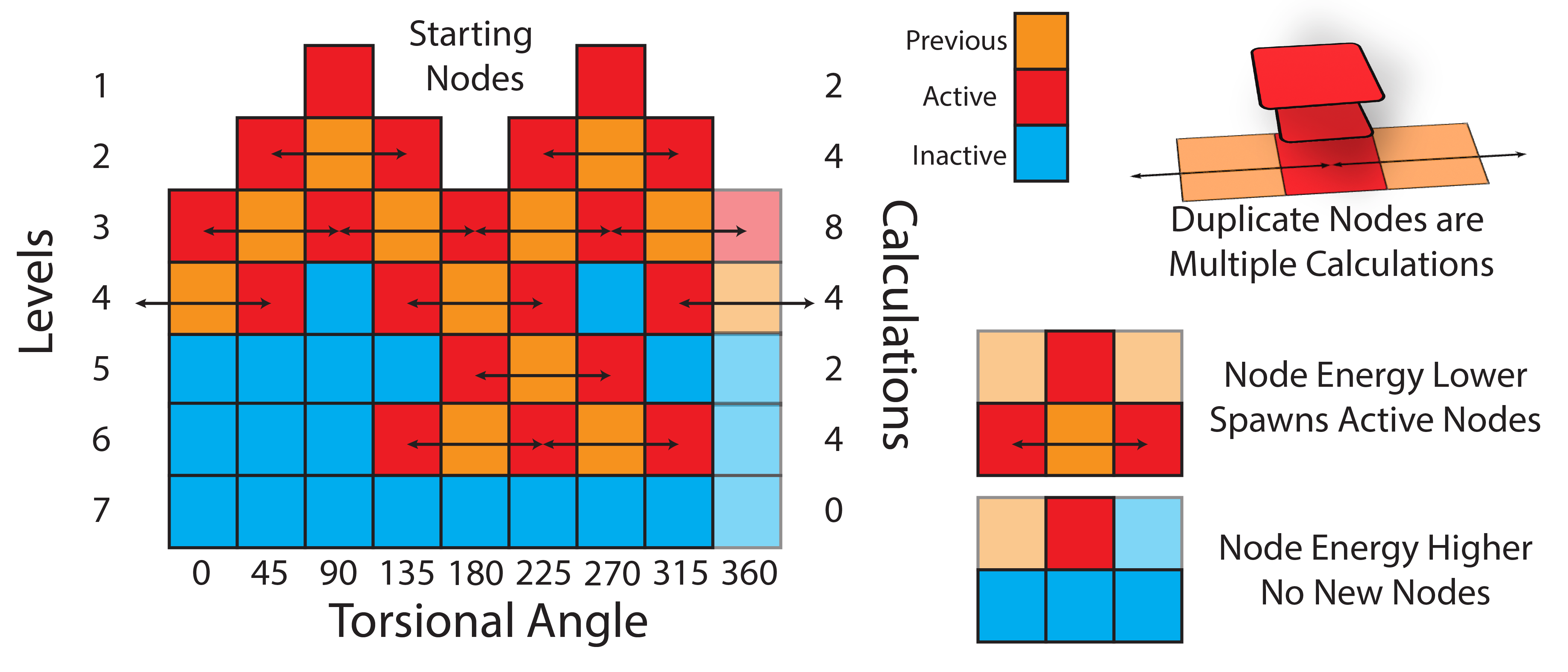
This often leads to many more total calculations; however, due to the parallelizability of each level of the scan, this is often significantly faster than a traditional linear scan.