CPPTRAJ for Analysis
Learning Objectives
Activities
Introduction to CPPTRAJ
CPPTRAJ is a valuable asset to complement your computational toolkit, as this AMBER program can be used to achieve a more rigorus analysis of MD trajectories. In this section, you will learn how to use CPPTRAJ to wrap trajectories, calculate RMSDs/RMSFs, and find an average structure from a trajectory. For this activity, you will be given multiple CPPTRAJ input files. Each input file contains lines of commands for CPPTRAJ, but they can each be individually submitted in the interactive command line of CPPTRAJ. The interactive command line of CPPTRAJ can be accessed by typing into your terminal:
[user@local] cpptraj
Which will open up the interactive command line seen below:
[user@local] cpptraj
CPPTRAJ: Trajectory Analysis. V4.26.4 (AmberTools V20.00)
  ___  ___  ___  ___
   | \/ | \/ | \/ |
  _|_/\_|_/\_|_/\_|_


| Date/time: 00/00/26 00:00:00
| Available memory: 54.268 GB
To exit CPPTRAJ, simply type: quit.
Wrapping Trajectories
We will once again return to the MTR1 system. Before you start the analysis of a trajectory, you must first wrap the system. Wrapping a trajectory means adjusting the positions of the molecules in a simulation so that they can stay within your defined simulation box. If you were to open an unwrapped trajectory in VMD, you would see that the molecules within the system can appear to look separated, drifting away or blown out due to the periodic boundary conditions. Therefore, it can be hard to gain an accurate interpretation of what is true behavior displayed in your system. If you are wanting to visually inspect your system, wrapping should be the first step prior to trajectory analysis to avoid confusion.
Wrapping is one of CPPTRAJ’s most utilized roles. CPPTRAJ can wrap both restart files and trajectory files. In this case, you will be wrapping a MTR1 trajectory file. First, you must decide on a center in which to wrap everything around. It is a good practice to center your system around the solute, or you can be more specific and choose the catalytic center residues or a ligand.
add directory Access the CPPTRAJ interactive command line:
cpptraj
Like VMD, you must load the topology file first, followed by the trajectory or restart file. CPPTRAJ’s command to load a topology file is parm.
> parm topology.parm7
Note
You could also try typing the following into your terminal to load the topology file:
parm -p topology.parm7
Once CPPTRAJ loads, you’ll be at the interactive prompt. Load your trajectory file using the trajin command:
trajin trajectory.nc
Note
Windows Users: load DCD trajectory file.
Now apply the wrapping commands. The basic wrapping workflow uses the reference, center and image commands. The reference command specifies the reference structure for centering and imaging. The center command moves the center of mass of the specified group to the origin, and the image command re-images all other molecules into the primary periodic box based on this centered group.
For MTR1, you will be centering around the solute. A typical mask for the solute can be described as :
solute='!@H= & !:MG= & !:NA= & !:CL= & !:PB= & !:WAT='
This mask selects all atoms that are not hydrogens, water, nor magnesium, sodium, chlorine, or lead ions. Use this mask to center your system around the solute. Essentially, it tells cpptraj to center the system around the heavy atoms of the solute.
Note
The symbols used in the mask have specific meanings:
@— Refers toatom names:— Refers toresidue names!— LogicalNOT(exclude)&— LogicalAND=— Wildcard (matches anything that begins with the preceding text)
Type the following commands into the CPPTRAJ interactive command line to wrap your trajectory:
reference MTR1.rst7
center '!@H= & !:MG= & !:NA= & !:CL= & !:PB= & !:WAT=' mass origin
autoimage '!@H= & !:MG= & !:NA= & !:CL= & !:PB= & !:WAT='
center '!@H= & !:MG= & !:NA= & !:CL= & !:PB= & !:WAT=' mass reference
Note
The atom selection syntax in CPPTRAJ might take some time getting use to.
massindicates that the centering should be done based on the center of mass of the atom selection.autoimageautomatically re-image coordinates.originmeans that the center of mass will be moved to the origin (0,0,0) of the coordinate system.
To write out the wrapped trajectory:
trajout centered.MTR1.nc
Execute the commands by typing:
run
or
go
The wrapped trajectory will now be saved. Once the job is finished running, type quit to exit CPPTRAJ and the interactive command line. You can visualize this in VMD to see that the system appears intact with all molecules properly positioned within the box around your solute of interest, or in this case, MTR1.
Your cpptraj interactive command line should look something like this:
[user@local] cpptraj


CPPTRAJ: Trajectory Analysis. V4.26.4 (AmberTools V20.00)
    ___  ___  ___  ___
     | \/ | \/ | \/ |
    _|_/\_|_/\_|_/\_|_

| Date/time: 00/00/26 16:49:33
| Available memory: 27.131 GB

  Loading previous history from log 'cpptraj.log'
> parm MTR1_prot-run.parm7
  [parm MTR1_prot-run.parm7]
  Reading 'MTR1_prot-run.parm7' as Amber Topology
  Radius Set: modified Bondi radii (mbondi)
> trajin MTR1_prot-run.nc
  [trajin MTR1_prot-run.nc]
  Reading 'MTR1_prot-run.nc' as Amber NetCDF
> reference MTR1_prot-run.rst7
  [reference MTR1_prot-run.rst7]
  Reading 'MTR1_prot-run.rst7' as Amber Restart
  Setting active reference for distance-based masks:       'MTR1_prot-run.rst7'
> center '!@H= & !:MG= & !:NA= & !:CL= & !:PB= & !:WAT='       mass origin
  [center '!@H= & !:MG= & !:NA= & !:CL= & !:PB= & !:WAT='      mass origin]
    CENTER: Centering coordinates using center of mass of      atoms in mask (!@H* & !:MG* & !:NA* & !:CL* & !:PB* &    !:WAT*) to
  coordinate origin.
> autoimage '!@H= & !:MG= & !:NA= & !:CL= & !:PB= & !:WAT='
  [autoimage '!@H= & !:MG= & !:NA= & !:CL= & !:PB= &     !:WAT=']
    AUTOIMAGE: To box center based on center of mass,       anchor mask is [!@H= & !:MG= & !:NA= & !:CL= & !:PB= &      !:WAT=]
> center '!@H= & !:MG= & !:NA= & !:CL= & !:PB= & !:WAT='       mass reference
  [center '!@H= & !:MG= & !:NA= & !:CL= & !:PB= & !:WAT='      mass reference]
    CENTER: Centering coordinates using center of mass of      atoms in mask (!@H* & !:MG* & !:NA* & !:CL* & !:PB* &    !:WAT*) to
  center of mask (!@H* & !:MG* & !:NA* & !:CL* & !:PB* &      !:WAT*) in reference 'MTR1_prot-run.rst7'.
> trajout centered.MTR1_prot-run.nc
  [trajout centered.MTR1_prot-run.nc
  Writing 'centered.MTR1_prot-run.nc' as Amber NetCDF
> go
  [go]
---------- RUN BEGIN       -------------------------------------------------

PARAMETER FILES (1 total):
 0: MTR1_prot-run.parm7, 72443 atoms, 17745 res, box:       Trunc. Oct., 17678 mol, 17520 solvent

INPUT TRAJECTORIES (1 total):
 0: 'MTR1_prot-run.nc' is a NetCDF AMBER trajectory with       coordinates, time, box, Parm MTR1_prot-run.parm7 (Trunc.       Oct. box) (reading 100 of 100)
  Coordinate processing will occur on 100 frames.

REFERENCE FRAMES (1 total):
    0: centered.MTR1_prot-run.rst7:1
  Active reference frame for distance-based masks is       'Cpptraj Generated Restart'

OUTPUT TRAJECTORIES (1 total):
  'centered.MTR1_prot-run.nc' (100 frames) is a NetCDF AMBER      trajectory

BEGIN TRAJECTORY PROCESSING:
.....................................................
ACTION SETUP FOR PARM 'MTR1_prot-run.parm7' (4 actions):
  0: [center !@H= & !:MG= & !:NA= & !:CL= & !:PB= & !:WAT=     mass origin]
  Mask [!@H*] corresponds to 36655 atoms.
  1: [center '!@H= & !:MG= & !:NA= & !:CL= & !:PB= &     !:WAT=' mass origin]
  Mask [!@H* & !:MG* & !:NA* & !:CL* & !:PB* & !:WAT*]     corresponds to 1459 atoms.
  2: [autoimage '!@H= & !:MG= & !:NA= & !:CL= & !:PB= &     !:WAT=']
  Original box is truncated octahedron, turning on      'familiar'.
  Anchoring on atoms selected by mask '!@H= & !:MG= &      !:NA= & !:CL= & !:PB= & !:WAT='
  Mask [!@H* & !:MG* & !:NA* & !:CL* & !:PB* & !:WAT*]     corresponds to 1459 atoms.
  2 molecules are fixed to anchor: 1 2
  17676 molecules are mobile.
  3: [center '!@H= & !:MG= & !:NA= & !:CL= & !:PB= &     !:WAT=' mass reference]
  Mask [!@H* & !:MG* & !:NA* & !:CL* & !:PB* & !:WAT*]     corresponds to 1459 atoms.
.....................................................
ACTIVE OUTPUT TRAJECTORIES (1):
  test.centered.nc (coordinates, time, box)
----- MTR1_prot-run.nc (1-100, 1) -----
 0% 10% 20% 30% 40% 51% 61% 71% 81% 91% 100% Complete.

Read 100 frames and processed 100 frames.
TIME: Avg. throughput= 37.8181 frames / second.

ACTION OUTPUT:
TIME: Analyses took 0.0000 seconds.

RUN TIMING:
TIME:             Init               : 0.0001 s (  0.01%)
TIME:             Trajectory Process : 2.6442 s ( 99.99%)
TIME:             Action Post        : 0.0000 s (  0.00%)
TIME:             Analysis           : 0.0000 s (  0.00%)
TIME:             Data File Write    : 0.0000 s (  0.00%)
TIME:             Other              : 0.0001 s (  0.00%)
TIME:     Run Total 2.6444 s
---------- RUN END      ---------------------------------------------------
> quit
  [quit]
\-----------------------------------------------------------      ---------------------
To cite CPPTRAJ use:
Daniel R. Roe and Thomas E. Cheatham, III, "PTRAJ and       CPPTRAJ: Software for
  Processing and Analysis of Molecular Dynamics Trajectory     Data". J. Chem.
  Theory Comput., 2013, 9 (7), pp 3084-3095.
The commands can be contained in a bash script to automate the process, and can be submitted by:
cpptraj -i wrap.in
With the script looking like:
#!/bin/bash

# Set Variables #

parFile=MTR1_prot-run.parm7
restartFile=MTR1_prot-run.rst7
trajFile=MTR1_prot-run.nc

# Define Solute Mask #
solute='!@H= & !:MG= & !:NA= & !:CL= & !:PB= & !:WAT='

# Write CPPTRAJ input file #
cat <<EOF > wrap.in
parm ${parFile}
trajin ${trajFile}
reference ${restartFile}
center '${solute}' mass origin
autoimage '${solute}'
center '${solute}' mass reference
trajout centered.${trajFile}
run
quit
EOF

# Run input file to wrap trajectory #
cpptraj -i wrap.in > c.log
rm c.log
Computing Average Structures and Fluctuations
You have already learned how to create RMSD plots using VMD. CPPTRAJ also has the capability to calculate RMSDs, but it can also calculate RMSFs and average structures.
In directory you will find the input script called. It looks like this:
parm MTR1_prot-run.parm7
trajin centered.MTR1_prot-run.nc
rms ToFirst :1-69&!@H= first out RMSD_MTR1.dat mass
run
quit
This input file again follows a standard of inputting your topology file first, then your trajectory. The rms ToFirst :1-69&!@H= first out RMSD_MTR1.dat mass line tells cpptraj to do an RMSD calculation, saving the data set as “ToFirst”, using all non-hydrogen atoms in the residues 1 through 69. This residue selection is the entire nucleic molecule. The first is telling cpptraj to use the first frame in the trajectory as a reference, with out as the command to write the output to a file named RMSD_MTR1.dat. The mass command indicates a mass-weighted RMSD calculation. Submit this file as your did before:
[user@local] cpptraj -i ctraj.RMSD_MTR1.in
Once the job is complete, the RMSD_MTR1.dat file will be in your
directory.
Using xmgrace, open this file:
[user@local] xmgrace RMSD_MTR1.dat
Which will pop up:
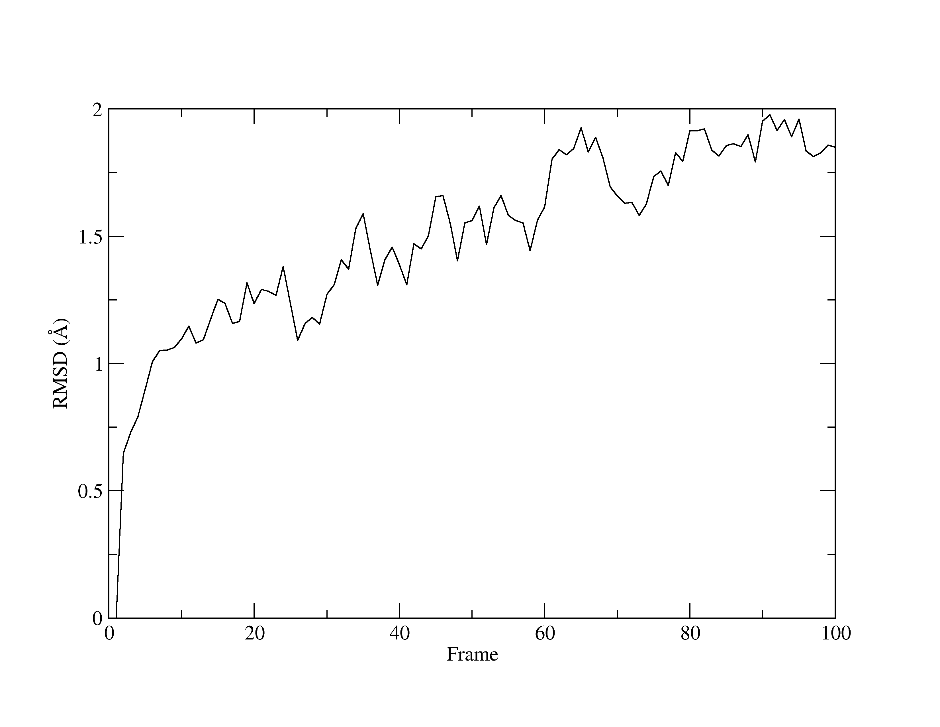
Figure 1. RMSD of MTR1.
With a quick glance of the graph, you will see that it is comparable to the same graph that was produced by VMD. Once again, the line fluctuates and has an upwards direction. Yet, given the very low values for RMSD, you can concur that the structure is stable.
Next, you will learn to use CPPTRAJ to calculate a Root Mean Square Fluctuation (RMSF). Like RMSDs, RMSFs are important analytical measurements that provide insight into your system. RMSFs quantify the overall flexibility and mobility of each atom or residue within your system as the simulation progresses. RMSFs calculate how much the position of each atom in your selection deviates from its average position throughout the simulation time.
In your directory, find the input file, ctraj.RMSF_MTR1.in.
Open in VIM to see the script:
parm MTR1_prot-run.parm7
reference centered.MTR1_prot-run.rst7
trajin centered.MTR1_prot-run.nc
rms :1-69&!@H reference mass
atomicfluct out RMSF_MTR1.dat :1-69&!@H= byres
atomicfluct out RMSF_Bfact_MTR1.dat :1-69&!@H= byres bfactor
run
quit
The script is similar to the previous one, but there are two new lines containing the RMSF commands. atomicfluct out RMSF.dat :1-69&!@H= byres and atomicfluct out RMSF_Bfact.dat :1-69&!@H= byres bfactor. atomicfluct is the command for an RMSF calculation. As seen before, out directs CPPTRAJ to output the data into a file name of your choosing (here, it is RMSF.dat, followed by your atom selection. The keyword byres specifies the output to be per residue, which sums the fluctuations of all atoms in each residue. The other keyword seen, bfactor, which will calculate the B-factor of the MD trajectory. This is an additional analysis one can do to compare simulation to crystallographic data. A low B-factor is indicative of a well-ordered and stable structure, while a high b-factor suggests more movement and thereby, greater fluctuations.
Open the RMSF.dat by using xmgrace:
[user@local] xmgrace RMSF_MTR1.dat
Which will look like this:
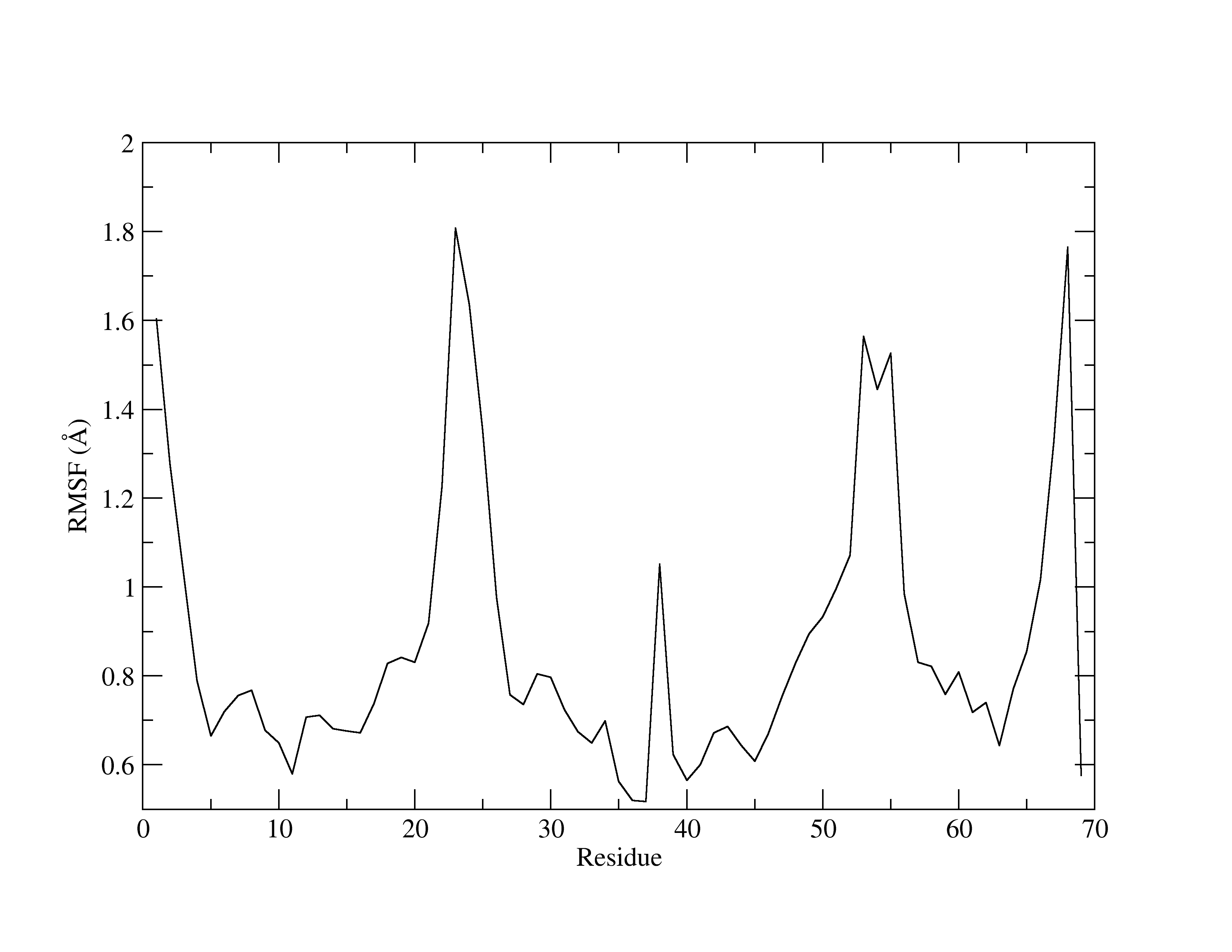
Figure 2. RMSF of MTR1.
Te x-axis is the residue number, while the y-axis shows the fluctuations (in Å). Higher peaks indicate greater fluctuations. RMSFs are useful for identifying residues that have a greater contribution to the overall dynamics of the structure. Usually, it is common for residues involved in crystal contacts to exhibit higher peaks, reflecting increased mobility.
Lastly, you will learn to obtain the average structure of a trajectory
using CPPTRAJ with the command average.
Find the input file ctraj.average_MTR1.in and VIM it.
parm MTR1_prot-run.parm7
trajin centered.MTR1_prot-run.nc
average avg.pdb :1-69&!@H= pdb
run
quit
After the average command, you must provide a filename in which to save the data. Here, the name is avg.pdb, followed by the atom selection mask and the PDB file type specification pdb.
Run the input file as usual:
[user@local] cpptraj -i ctraj.average_MTR1.in
Now, you have an average structure of MTR1 in a PDB format that can be opened up in VMD for viewing.