VMD Basics for Visualization
Learning Objectives
Learn the basic commands and interface of VMD necessary for exploring 3D molecular structures.
Master tools to visually inspect molecular properties, including bond distances, angles, and dihedral measurements.
Create and customize molecular representations to highlight specific structural features.
Perform trajectory analysis including RMSD calculations and interpretation.
Generate high-quality rendered images for scientific presentations and publications.
Apply selection syntax to identify and visualize protein-ligand interactions and hydrogen bonding patterns.
Activities
VMD
VMD is a powerful high-performance, cross-platform molecular graphics viewer developed by the Theoretical and Computational Biophysics Group (TCBG) that is widely used for displaying static and dynamic structures, viewing sequence information, and performing dynamic analysis. There is an online User’s Guide as well as a number of detailed activities available. Further support is provided by the VMD Mailing List.
Install on your Local Computer:
Download from this link here. Once downloaded, you can open VMD through the icon.
Note
If you are having trouble using VMD on a Windows machine: You can install Ubuntu as a Windows subsystem for Linux (WSL) and install VMD there. A quick guide to do so can be found here.
This activity will introduce you to the following systems:
MTR1 (ribozyme)
TYK2 (protein)
Note
All of the input files for this activity can be found in put in file placement. Please copy them to your working directory. Additionally, all output files produced by this activity can be found in put in file placemenmt should you need to access them.
You will begin by loading the Methyl-transferase (MTR1) ribozyme. More detailed information on this system will be explained in other activities (link), but for now, this is an RNA enzyme selected in vitro to catalyze the transfer of a methyl group from an exogenous O6-methylguanine (O6mG) to a target N1 of an adenine. It is a two step mechanism involving a proton transfer followed by a methyl transfer. The catalytic center of MTR1 is made up of residues 9, 44, 62 and 69. Residues 9, 44 and 62 are a protonated cytosine, uracil and adenine respectively, while residue 69 is the O6-methylguanine (O6mG) substrate.
Open VMD
Find the VMD Main window:
Main Menu→File→New Molecule→BrowseLoad you files: MTR1.pdb by selecting and press
Load.
The following will pop up:
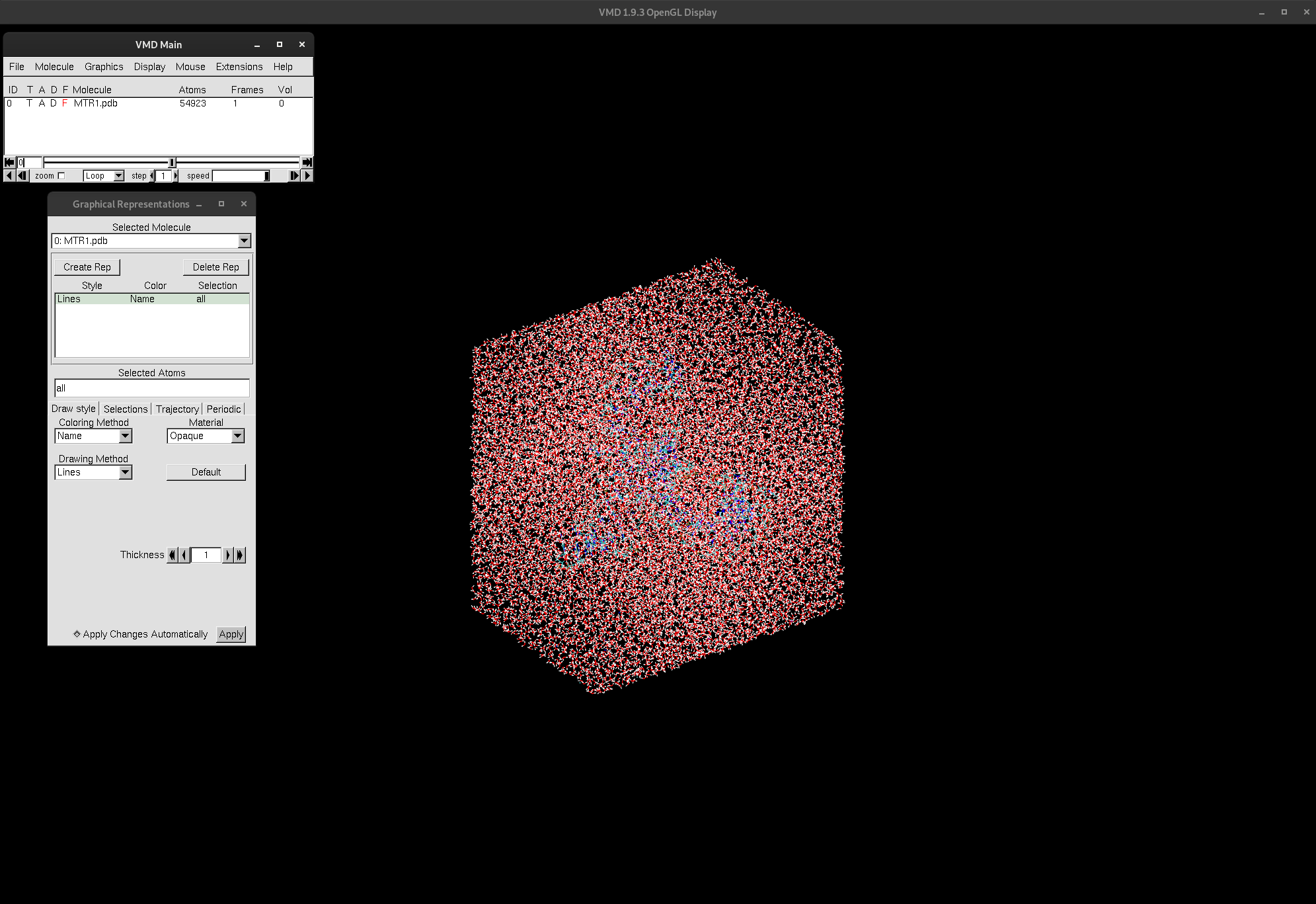
Figure 1. VMD display windows and MTR1 loaded.
As you can see, VMD consists of 3 windows:
Display
VMD Main
Graphical Representations
The VMD Main is the control window for VMD. Here, you will also be able to see which molecules are currently loaded in VMD. Next to each loaded molecule is a unique interger ID, along with T, A, D, and F. T stands for Top, A stands for Active (if this is on, commands will do their action for all the active molecules), and D stands for Drawn (if this is on, the molecule is being displayed). F stands for Frozen (if this is on, the molecule will not be affected by any mouse movements). You can toggle these options on or off by clicking on them.
In the VMD Main, you can also see the number of frames loaded (if a trajectory is loaded), the number of atoms, and the type of file that was loaded.
Tip
VMD contains a lot of gadgets and options for visualization and analysis, so carefully float your mouse over each menu option in the VMD Main to briefly explore the sub-menus. For example,if you go into the Display menu, you can change the settings of the display. Play around with different settings to see how it affects how the system is displayed. This is up to the user’s preference.
Moving the molecule around in VMD is quite easy; you have the option of
going through the Mouse menu, or through keyboard shortcuts:
To rotate molecule:
rTo translate molecule:
tTo scale (zoom-in or out):
sTo center the system in the display:
=
Customizing Representations
Representations are used to separate out the individual components
within the system, such as distinguishing a ribozyme (solute) from
the surrounding waters and ions (solvent).
Under the Graphics menu, click on Representations.
Note
The Graphical Representations window is typically already up on your screen, but if it is not, selecting it will cause it to appear. This window provides a wide range of different ways to visually represent the molecules in your system, allowing for a more meaningful analysis of the structural organization and interactions.
In the Graphical Representations window, take time to look over the
different components.
At the top, you can see which system is selected. If you have multiple systems loaded, you can use the down arrow to toggle through them and view the representations for each system. For now, we only have one system loaded. There are two buttons under Create Rep and Delete Rep. The Create Rep will create a new representation, while the Delete Rep will delete. If you want to simply turn off a representation, double-click on the representation. It will turn red and be off. The Selected Atoms box is where you type what will be your selection for the representation at hand. Underneath that are four tabs:
Draw style
Selections
Trajectory
Periodic
Draw style is where you have the creative ability to change how the selection is represented. The Coloring Method is where you define how the colors are assigned to molecules. The Drawing Method determines the shapes of its atoms, bonds and other components. And the Material can change shading or how the objects appear. The default representation selection is all. If you need additional guidance on the available selection types, the Selections tab provides a list of options that you can browse. When a trajectory is loaded into VMD, you can smooth the animation by changing the settings under the Trajectory tab. Lastly, the Periodic tab is a good place to check if your periodic unit cell box is properly established. Here you can display multiple unit cells.
To make our first representation:
Make a new representation by clicking
Create RepType
all not water.Turn off the other representation
all.
You should see now that only the ions and MTR1 are selected and displayed:
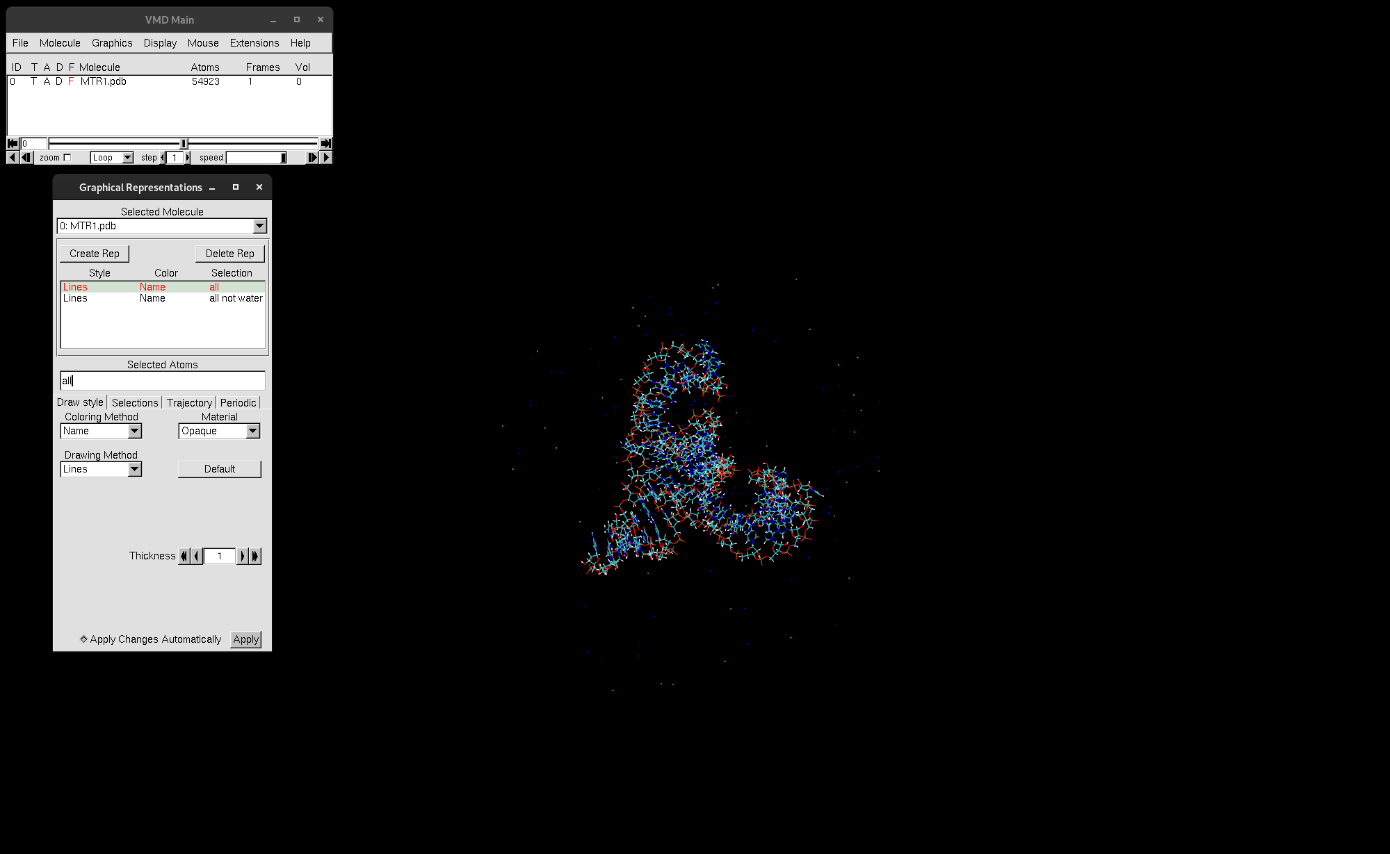
Figure 2. Representation all not water displayed.
Now, we will create representations to select the residues that make up the catalytic center of MTR1. First:
Create a new representation and type
all not solvent.Change the
Drawing MethodtoLicorice.Turn off the other representations.
Press
=to reorient the screen to your selection.
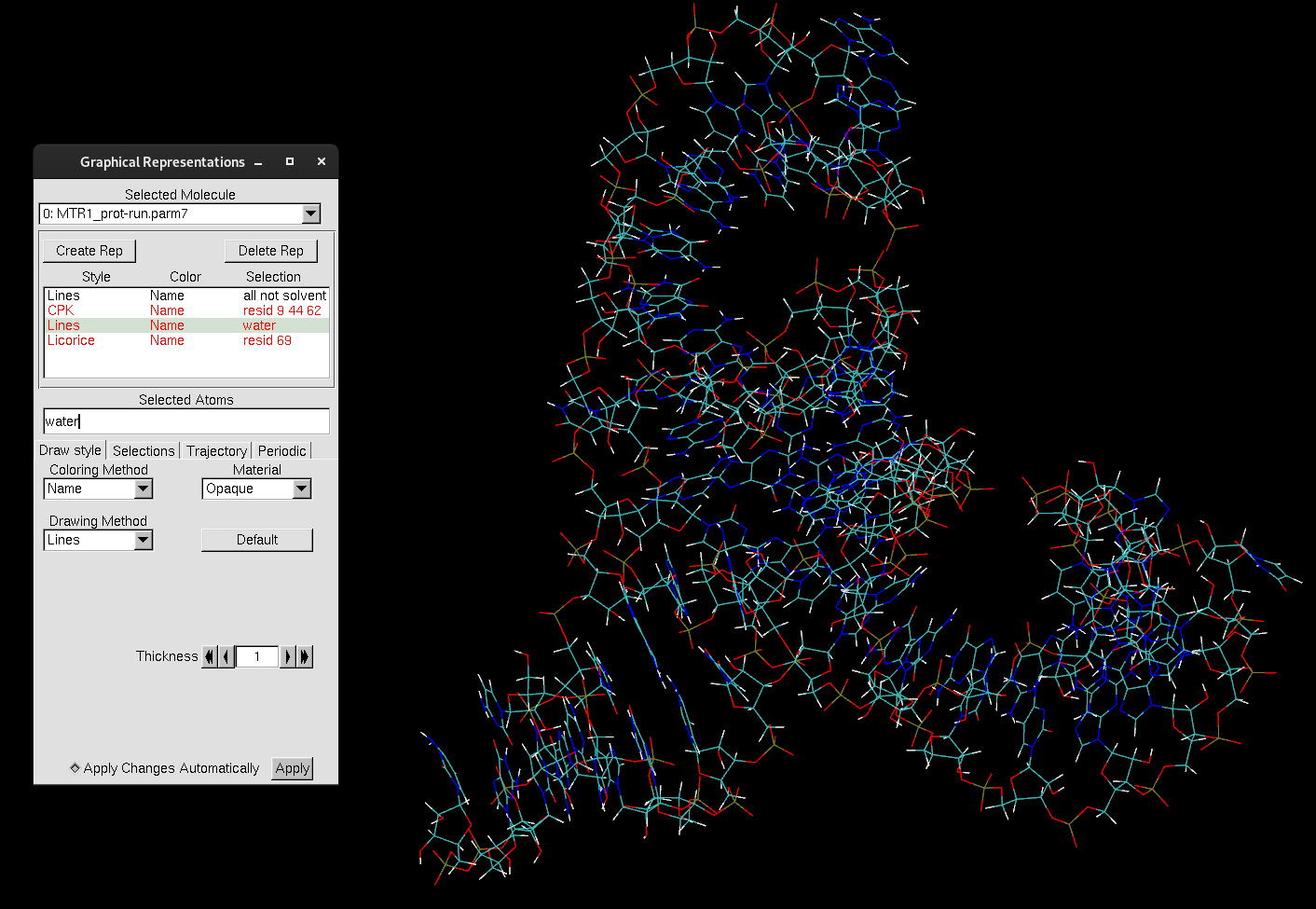
Figure 3. MTR1.
- Now, to select the catalytic center residues:
Create a new representation and type
resid 9 44 62 and not water.Change the
Drawing MethodtoCPK.Create a new representation and type
resid 69 and not water.Change the
Drawing MethodtoLicorice.Turn off the other representations.
Press
=to reorient the screen to your selection.
You should now see the catalytic center residues highlighted in different representations. Residues 9, 44 and 62 are a protonated cytosine, uracil and adenine respectively, while residue 69 is the O6-methylguanine (O6mG) substrate.
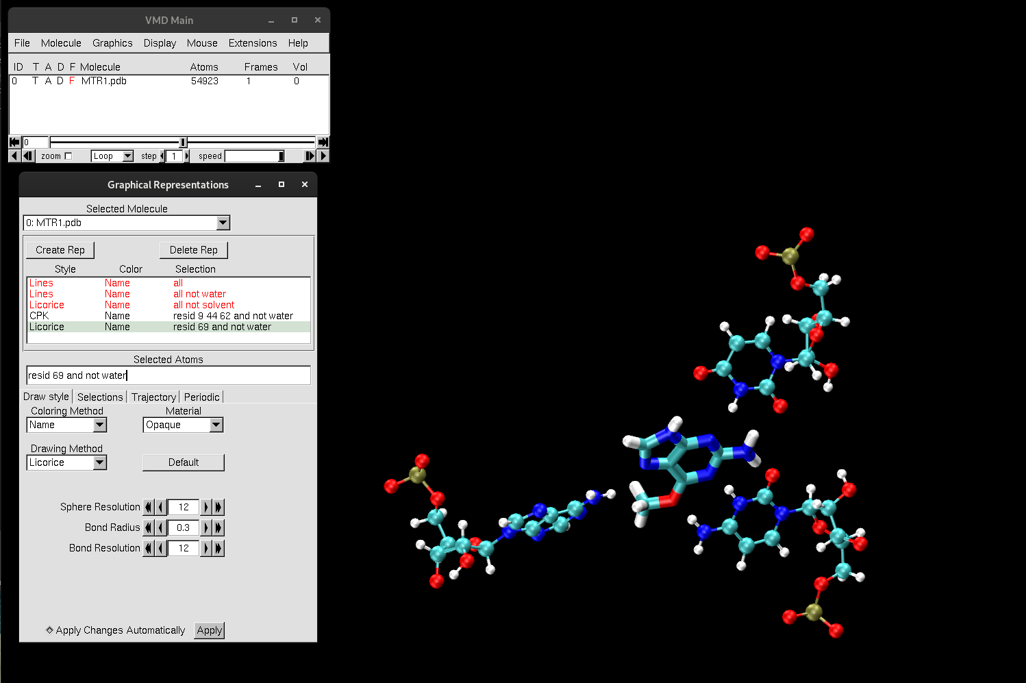
Figure 4. Catalytic center of MTR1.
Measuring Geometrical Properties
Next, find the Mouse menu in VMD Main. Go to the sub-menu, and find Label.
Here, you can switch-on selection modes to label atoms, bonds or angles in order to obtain metrics about the system. You can either use the selections seen in the sub-menu or you can use these keyboard shortcuts:
To select an atom, press
1and then make your selection. It will add a label that contains the residue ID and the atom name.To select and measure a bond distance between two atoms, press
2. First click on one atom, then click on the other. The distance between the two atoms will pop up in Å.To select and measure an angle, press
3and carefully select three atoms of choice. A label for the angle will be displayed.To select and measure a dihedral angle between four atoms, press
4and carefully select the atoms. A label for the angle will be displayed.
Tip
You should get very comfortable switching between the different selection types using the keyboard.
Try adding a label to some of the atoms of each residue:
Press
1on the keyboard and label an atom within the molecule. If labels are not showing up, try zooming out first.Rotate the molecule to see the labels.
See if you can locate the following atoms:
the nucleophile (N1 of residue 62)
the electrophilic carbon (C6 within the methyl group of residue 69)
the protonated cytosine site (cytosine is protonated at the N3 position)
Once you have found these atoms, try to measure the distance between the nucleophile and electrophile (press 2 to initiate bond distance, and find A62:N1 and 69:H6), the bond distance between the protonated cytosine site and the substrate (C9:N3 and 69:N3) and the angle of the atoms involved in the proton transferring from cytosine to the substrate (C9:N3, 69:H13 and 69:N3).
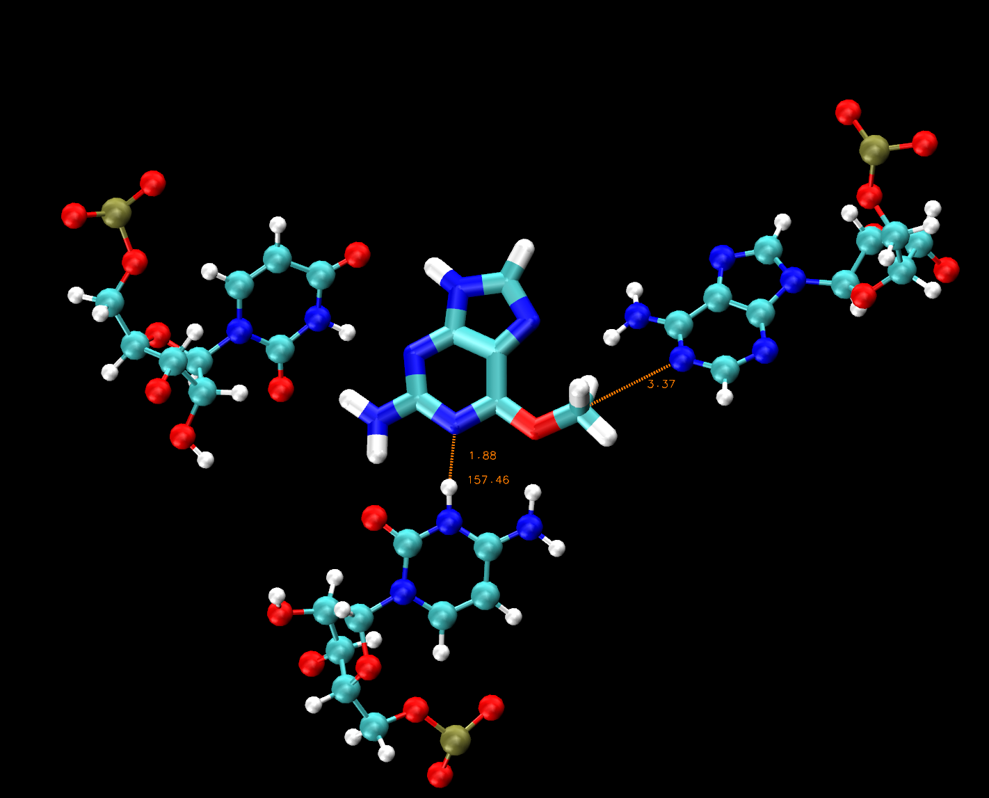
Figure 5. Example of distance and angle measurements in VMD for MTR1.
All of the labels that you create are stored under Graphics → Labels. Here, you can find more specifications regarding the atom, bond or angle that you had labeled. For example, you can see what residue a labeled atom belongs to, turn labels on or off, or remove labels completely. Feel free to explore this window and all of its different components.
Selections with within and same
Learning how to create meaningful representations in VMD that can capture exactly what you need takes time and practice. However, there are a few tricks to quickly and efficiently select your desired components. A helpful keyword for selecting and finding atoms within a certain distance is within. This is an essential element to include in your atom selection when you want a fast way to narrow down certain interactions, distances or spatial relationships.
Create a new representation:
water within 3 of resid 69.
This selection will select the atoms of water that are within 3 Å of residue 69. You can adjust the distance cutoff to be more or less stringent. This is a quick way to find potential interactions between the substrate and the surrounding solvent. However, you may have noticed that some water molecules are only partially selected, meaning that only some of the atoms of the water molecule are within 3 Å of residue 69.
If you want to select the entire water molecule, you can use the keyword same This keyword groups atoms together based on shared properties. For example, you can type same chain as resname ALA, or same residue as name O. Both of these keywords will become clearer as you implement them.
Create a new representation:
same residue as water within 3 of resid 69. Now, the entire water molecule will be selected if any of its atoms are within 3 Å of residue 69.
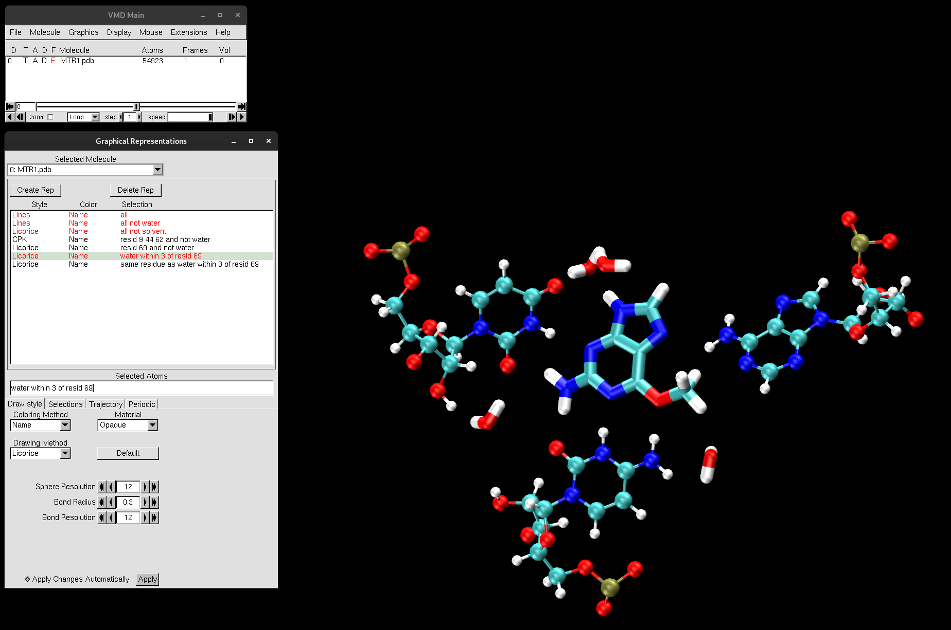
Figure 6. Water molecules within 3 Å of residue 69 and the catalytic center of MTR1.
Trajectory Analysis
Calculating Root-Mean-Square Deviation (RMSD)
Now, you will learn how to use VMD to calculate an RMSD. This time instead of loading a PDB file, you will now load a trajectory file of the MTR1 system. The trajectory is from an AMBER MD simulation, and this system will be used in the additional activities. In the directory INPUT, you will see the files obtained from MD simulations of the RNA enzyme system, MTR1. The files are MTR1_prot-run.parm7 and centered.MTR1_prot-run.nc (or with .dcd extension).
Open this trajectory by either starting a new VMD session (quitting your current session and restarting VMD), or opening it in the same VMD session.
To open the trajectory of MTR1 in the current session, you can follow the steps we took before for loading a system:
Main Menu→File→New Molecule→Browse.Find the parameter file MTR1_prot-run.parm7 and select.
Once selected, the
Determine file type:should readAMBER7 Parm.Press
Load.
Now, to load the trajectory file:
Browseagain and find centered.MTR1_prot-run.nc orcentered.MTR1_prot-run.dcdforWindows Users.Select it and press
Load.
If you are using the terminal to load a new VMD session:
[user@local] vmd MTR1_prot-run.parm7 centered.MTR1_prot-run.nc
Note
Larger trajectories may take longer to load into VMD.
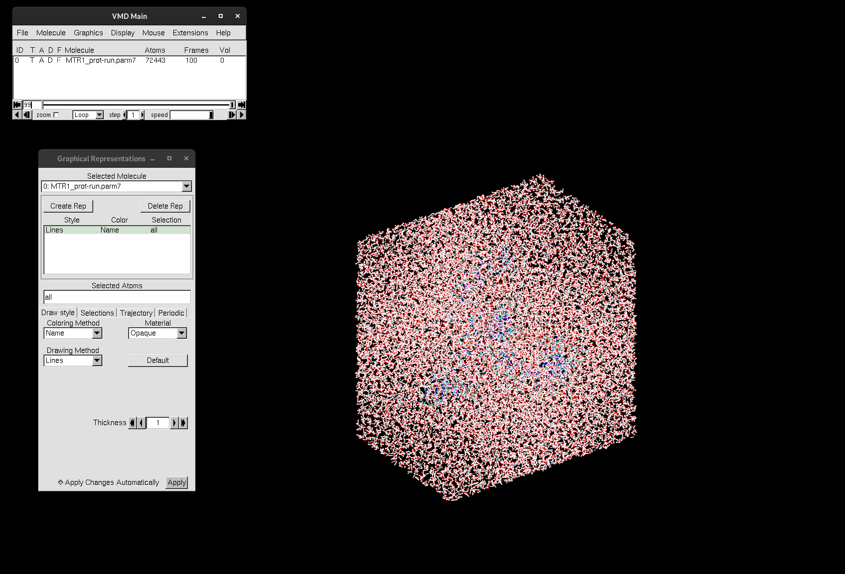
Figure 7. Trajectory file of MTR1 loaded into VMD.
If you decided to load both systems into one VMD session, you will now see in VMD Main that there are multiple molecules loaded. Now you have the option to remove the display of one by clicking the D next to the molecule. It will turn red, indicating that it is off. Additionally, the Graphical Representations window will have an option to toggle through systems to see their representations.
If you have multiple systems loaded in your VMD session, hide the first MTR1 PDB system so we can focus on the MTR1 trajectory.
With a trajectory now loaded, you can now make use of the animation toolbar at the bottom in VMD Main. The slider will transition through the frames, with the number to the left of the slider indicating which frame you are viewing. When first loaded, the trajectory will be at the last frame. You can also play the trajectory as an animation, change the speed of the animation and change the animation type (ex: Loop). To get started with our MTR1 trajectory analysis, create the following representations that you have seen before for the PDB structure:
all not solvent
resid 9 44 62
water
resid 69
Change the Drawing Method to match with the representations below:
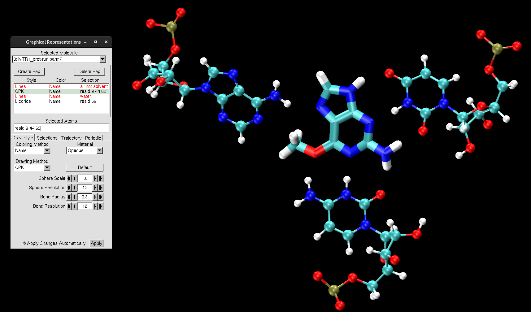
Figure 8. MTR1 representations to highlight the catalytic center.
As mentioned before, we will use VMD to calculate its Root Mean Square Deviation (RMSD). RMSDs are helpful in understanding how much the structure deviates from the original starting structure over the time of the simulation. This is an important metric to support if you have a stable structure or not.
To perform this analysis, turn off all representations besides all not solvent to isolate the catalytic center.
Access the RMSD Trajectory Tool by going to Extensions → Analysis → RMSD Trajectory Tool.
An interface will pop up. In the left white box, you can select the atoms (same way that you would make a representation) to select the region of the system you want to perform the RMSD calculation on. For example, the default is protein, which will perform the RMSD of the entire protein, if you were to have one.
For this system, replace protein with nucleic to select the entirety of the ribozyme. You can be more specific with your selection for an RMSD calculation, such as, typing resid 9 44 62 69. The tick boxes you see allows for quicker selections to add on:
Backbone: adds on atoms within the backbone.
Trace: adds ‘and name CA’.
noh: which will exclude hydrogens from the atom selection.
nohshould already be selected for you. Keep it selected.
Once you made your selection:
Press the
Alignbutton.
It is important to first align all the frames in the trajectory to your selection before calculating the RMSD. This is because if you do not align, the structure will jump all around as it switches frames, making it impossible to get a grasp on things.
You might see a shift in the structure, and that is VMD aligning the molecule to your selection (nucleic) from frame 1. If you have multiple structures loaded, you will see them in the table within the RMSD Trajectory Tool window. If this were the case, you decide which structure is the Reference mol and which structures to align to that.
After you have hit the Align button:
Press the
RMSDbutton.
The RMSD values for calculation will print in the table, including the average RMSD and the standard deviation.
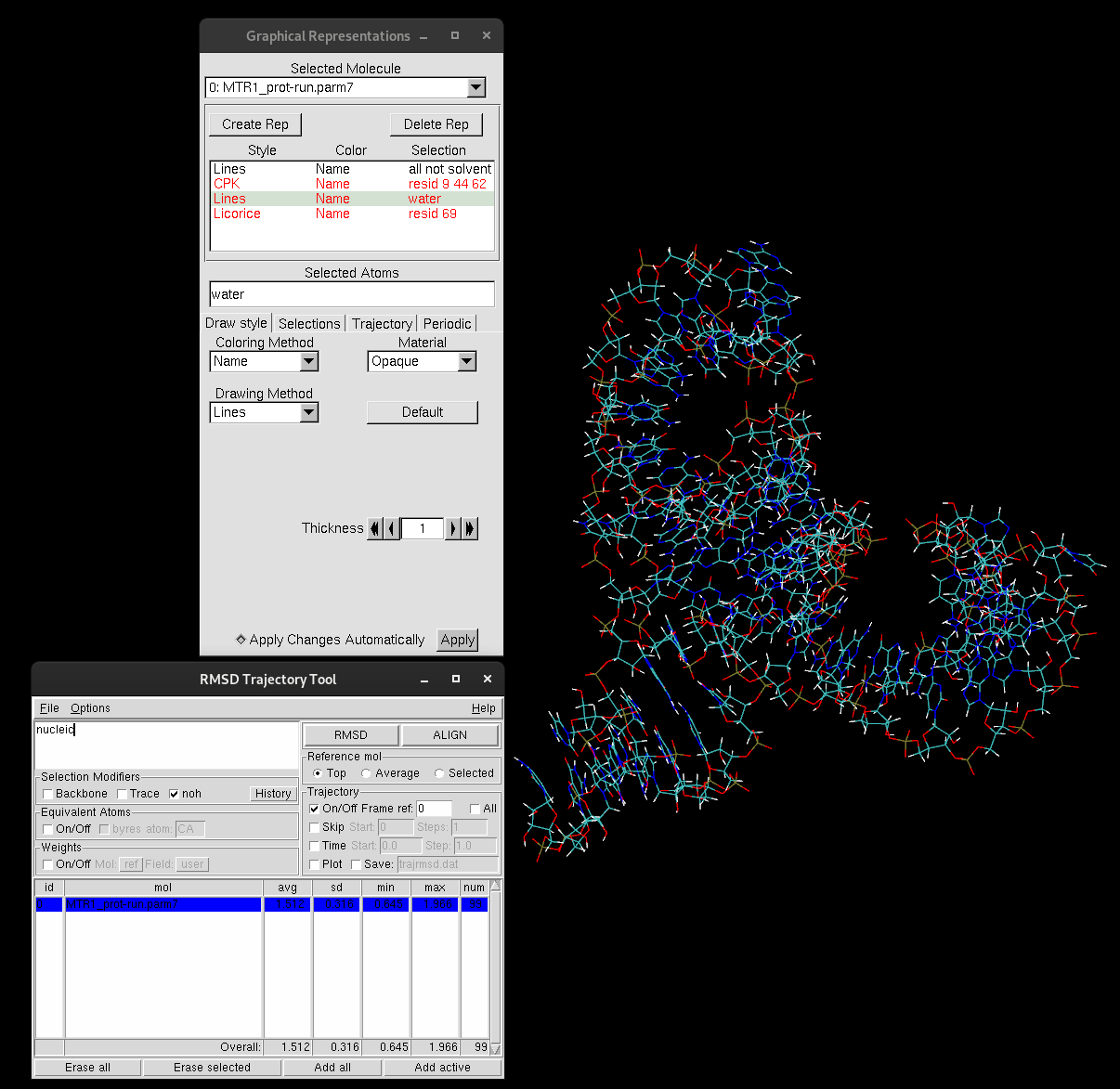
Figure 9. RMSD Trajectory Tool table.
To gain further insight into the meaning of the RMSD:
Tick the box
Plot, and clickRMSDagain.
The plot generated depicts the RMSD (in Å) with each frame of the trajectory. This plot provides valuable insights into the movement of your selection. High RMSD values should be noted, as that indicates that the molecule is undergoing significant structural changes. If the RMSD continues to climb, this is indicative of the structure either failing to reach equilibrium or that there is instability in the structure. If this were to be the case for you, it is suggested that you narrow down your selection to try and investigate which regions are responsible for the most change. In general, RMSDs tend to climb throughout the beginning of simulation, but there is a period in which it stabilizes. You must have a stable structure to depart from for further computation exploration.
Save the generated plot by ticking the Save box and click the RMSD button again. A trajrmsd.dat file will be produced.
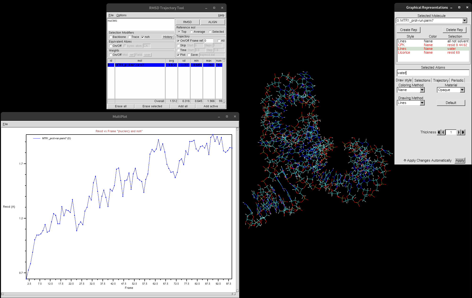
Figure 10. RMSD graph produced by RMSD Trajectory Tool.
As you can see, the RMSD is trending upwards, however, if you look at the value of Å, the RMSD is very low. This indicates the structure is quite stable.
Image Rendering
Another tool of VMD is to render high-quality images and animations of your system for posters, presentations or publications. We will quickly walk through the steps to obtain a high-quality image on this MTR1 system. First you must set up the scene that you want to display for your high-quality image:
Turn off all of the representations besides
all not solvent.Select
all not solvent, and change theDrawing MethodtoNewRibbons.Under
Material, change toEdgyShiny.
Think of rendering the image as taking a screenshot or snapshot, therefore adjusting the view by rotating or zooming in or out to obtain a full view of the ribozyme. We also do not want to have the axis on in our image:
Turn off the axis by navigating to the VMD Main window and selecting
Display→Axes→Off.
Next, you can change the projection mode:
From the
Displaymenu, selectPerspective.
VMD offers two projection modes including Perspective and Orthographic. The Perspective mode shows the structure with perspective, meaning objects further from the viewer appear smaller than those closer. This mode is useful for generating images. The Orthographic mode provides a uniform scale across the entire image, which is useful for trajectory analysis.
You can also turn the Depth Cueing on or off by:
Display→Depth Cueing.
This option provides a realistic 3D view with depth perception. You can also change the background color to white through:
Graphics→Colors.Select
Display→Backgroundunder theCategories.Scroll up till you see white, and select it.
Now, once you have the display to your liking, render the image by going to:
File→Render.
In the pop-up window, the default program used to render the image is Snapshot (VMD OpenGL window). This is low quality and not recommended for obtaining high-quality images. In the drop-down menu:
Select
Tachyon (internal, in-memory rendering.Change the filename and location for the image by clicking the
Browsebutton.Click the
Start Renderingbutton.
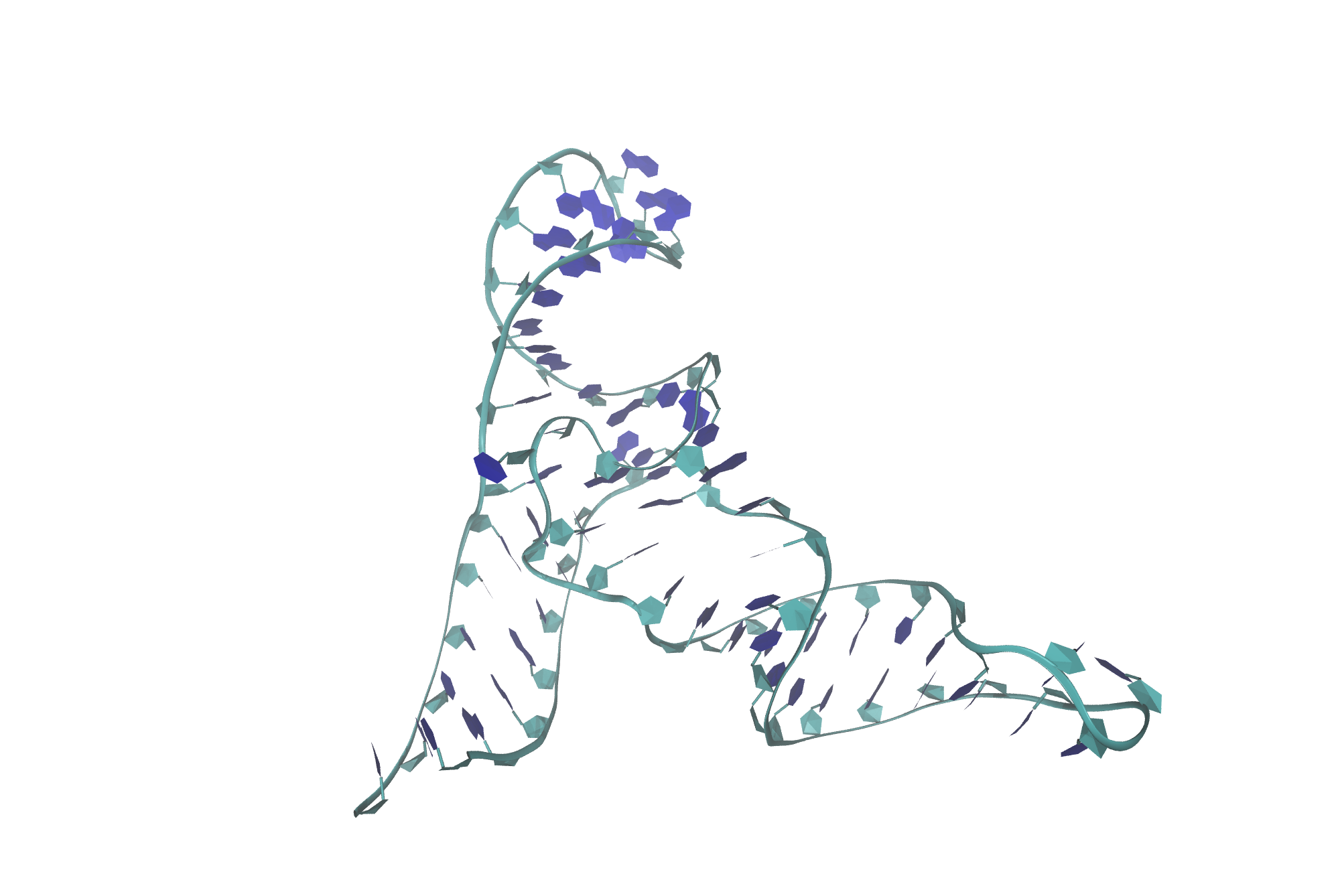
Figure 11. High-quality rendered image of MTR1.
Your high-quality image will pop up! If it is not to your liking, feel free to change the settings, adjust the view and render again.
Loading Multiple PDBs
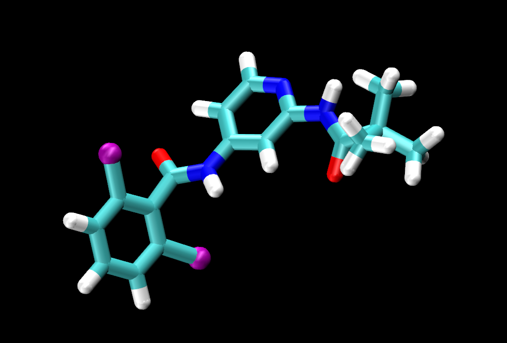
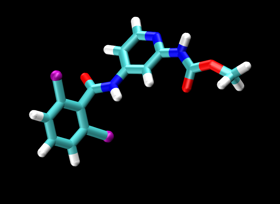
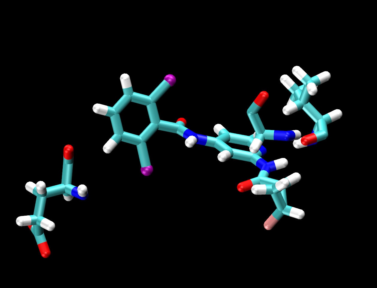
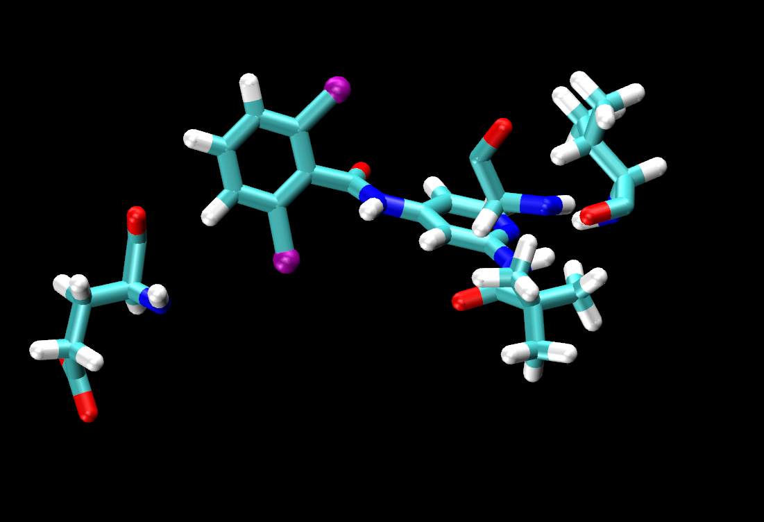
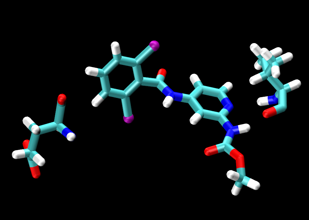
Now, you will be looking at the protein TYK2 with three chemically distinct ligands with differing compositions, L00 and L26. This system will be used for Alchemical Free Energy Simulations in future activities need to tag the tutorial, where you will calculate the relative free binding energies of the ligands bound to this protein.
Find the terminal once again to open the three systems at once:
[user@local] vmd -f jmc_23.pdb -f ejm_44.pdb -f ejm_55.pdb
Once loaded in VMD, you will see that there are three systems loaded, each with a unique integer ID. In the Graphical Representations window, toggle through the systems through the down arrow seen in Selected Molecules. For each molecule, created the following representations. It might be helpful to first turn off whichever system you are not working with (click on the D next to the system in VMD Main to turn it off):
protein
resname LIG
Change the
Drawing Methodofresname LIGtoLicoricefor all three systems.
Currently, the chlorine atoms in all three ligands are all colored the same as the carbons. To visually distinguish the chlorine atoms in the ligands, you can change their coloring:
Create a new representation of
name CL1 CL2Change the
Drawing MethodtoCPK.Change the
Coloring Method→ColorID→11for bothname CL1 CL2.
You could also change the color of the chlorine by Type by making a selection based on atom mass, mass 35.450001.
|
|
|
Visually inspect the three ligands. You should see that they are all the same except for the tail end of the ligand, where jmc_23 has CHANGE, ejm_44 has CHANGE and ejm_55 has CHANGE.
Hydrogen Bonding
Now, you are going to make use of those special keywords to observe hydrogen-bonding contacts between the ligands and the protein. Hydrogen bonding has the potential to be a factor in the binding affinity.
Add these representations with Licorice as the Drawing Method:
same residue as (name H and within 3 of resname LIG)
The selection in parentheses (name H and within 3 of resname LIG) will select the atoms that are within that distance. 3 Å is an appropriate distance cutoff to highlight potential hydrogen-bonding contacts. Based on the selection within the parentheses, the same residue as will select the entire residue that the selection in parentheses belongs to.
Moreover, if you were to just type the selection within the parentheses, you would see that only the atoms (not entire residues) of the protein that are within 3 Å of the ligand pop up. The
samekeyword will select the entire residue that pops up from that selection.Parentheses and keywords allow for flexible and efficient selections.
Turn off/on the representations pertaining to each ligand to examine the interaction and spatial arrangement of each ligand one at a time. You should notice that all ligands share the same number of hydrogen bonding contacts with VAL92.
|
|
|
You can use this type of technique to quickly visualize potential interactions between a ligand and its receptor. This is helpful in drug design to see how well a ligand is binding, and if there are any opportunities to improve binding through additional interactions.