Hands-On Session 5: Using QM and Machine Learning Potentials to Parameterize Torsion Terms for Flexible Molecules
Learning objectives
Understand the simplest command-line usage of LigandParam.
Learn how to use the LigandParam Python API for more complex tasks.
Use FFPOPT to Run Dihedral Scans for a Simple Molecule using the a Linear Scan Method
Use FFPOPT to Run Dihedral Scans for a Simple Molecule using the WaveFront Method
Relevant literature
Outline
In this tutorial, we will be using the python package LigandParam, developed by the York Group, to parameterize a ligand for use in molecular dynamics simulations. For this tutorial, we will be parameterizing the ligand…
Tutorial
Overview of Ligand Parameterization and Terminology
In most tutorials for the Amber Molecular Dynamics package, the first stage of that tutorial is running a ligand parameterization to determine the force field parameters for the ligand.
This is usually done as a multi-stage process, that usually involves some combination of the following steps:
Ligand Cleaning (by hand/script)
Atom Type Assignment with (Antechamber)
Initial BCC or ABCG2 Charge Assignment (Antechamber)
Electronic Structure Theory Geometry Optimization and RESP Charge Calculation (Gaussian)
RESP Charge Fitting (resp.F)
Charge Equalization (By hand/script)
Assignment of Bonded/Angle/Dihedral Parameters (Parmchk2)
Writing a lib file (tleap)
PDB Name Matching (By hand/script)
In a wide-range of scenarios, some or most of these steps are omitted in tutorials to streamline the parameterization process. This can lead to the scenario that tutorials are teaching methods that groups are not actually using to develop force-field parameters for ligands in reality. In the following section, we will outline the use of LigandParam, a software tool developed by the York group for making Ligand Parameterization easy to do in a way that matches our best practices.
With that said, before we show you the tool, there are a few important concepts that should be defined.
1. Atom Types: Atom types are the building blocks used by amber force-fields to assign interaction parameters within a molecule. These are usually specific to both chemical element and bonding environment. An sp3 carbon will get different parameters than an sp2 carbon, and so forth.
2. Charge Models: An important part of the force-field parameterization process is the assignment of partial atomic charges to the atoms in the ligand. These charges are used to describe the electrostatic interactions between atoms. There are a variety of charge models that can be used, including:
RESP (Restrained Electrostatic Potential) Fitting
AM1-BCC
ABCG2
The original (and often widely used) charge model is AM1-BCC - this is likely the one you will find in most tutorials. AMBER recently created a new charge model, called ABCG2, which has been shown to lead to improvements in things like solvation free energies. Lastly, RESP charges can be calculated from electronic structure theory calculations which provides the most accurate charges but at the highest-expense.
3. PDB Name Matching: This step involves ensuring that the atom names in the ligand’s PDB file match the atom names in the generated force-field files.This is necessary for making sure that the right atoms get the right parameters.
At the very simplest, a ligand parameterization can be done just with Antechamber, ParmChk2, tleap, as follows.
Start by creating a subdirectory called by_hand, and copy the ligand pdb into that subdirectory from your current working directory.
mkdir by_hand
cp ligand.pdb by_hand/
cd by_hand
Assume you are starting with ligand.pdb, first you would call antechamber to create a mol2 file with bcc charges.
antechamber -i ligand.pdb -o ligand.mol2 -fi pdb -fo mol2 -c bcc -rn LIG -at gaff2
The options here are:
-i: Input file (ligand.pdb)
-o: Output file (ligand.mol2)
-fi: Input file format (pdb)
-fo: Output file format (mol2)
-c: Charge method (bcc)
-rn: Residue name (LIG)
-at: Atom type (gaff2)
This command creates a mol2 file with BCC-assigned partial charges next to each atom.
parmchk2 -i ligand.mol2 -o ligand.frcmod -f mol2 -s 2
The options here are:
-i: Input file (ligand.mol2)
-o: Output file (ligand.frcmod)
-f: Input file format (mol2)
-s: ff parm set (2, which is equivalent to gaff2)
This creates a frcmod file from the above mol2 file, which is a file the stores bonded, angle, and dihedral parameters that are not found in the standard force-field. With each entry, there is a penalty field which describes how sure of the parameters the program is. The higher the value, the less confident in the parameters the program is.
Note
These are not the only parameters that describe bonded/angular/dihedral interactions - the standard forcefields have files shipped with amber that define their parameters (located in amber/data/leap/gaff2.dat for gaff2).
Now that we have base intramolecular force-field parameters, the last thing we need is a lib file. These files store those partial charges that we provided earlier so that if you are building a system from a docked structure you aren’t forced to re-generate a mol2 with the correct coordinates and can use a pdb instead.
Here is an example of that file.
source leaprc.gaff2
loadamberparams ligand.frcmod
LIG = loadmol2 ligand.mol2

saveOff LIG ligand.lib
quit
Now, we can run tleap on this file as:
tleap -f leap.in
Now this is an easy parameterization, and this already involves running three different programs: antechamber, parmchk2, and tleap. Now imagine you add in the by-hand adjustments described above, and also add in RESP charge fitting. It is pretty clear that this process can get complicated quickly, it is easy to make mistakes, and keeping track of all the different files and parameters can be challenging. There is a better way.
Parameterizing with LigandParam
Within the “York Group”, we have developed a tool called LigandParam that automates the above process and makes it easy to do ligand parameterization in a way that matches our best practices.
LigandParam is available by installing through pip with the following command:
pip install ligandparam
Warning
One should only ever install LigandParam into a virtual environment to avoid conflicts with other environments and to keep your base environment clean.
python -m venv ligandparam_env
source ligandparam_env/bin/activate
pip install ligandparam
Once installed, you now have LigandParam’s command line interface. LigandParam is a complex package, with a wide-range of tools aimed at helping to automate LigandParameterization with relatively little user input. It works by running a prebuilt set of recipes that at its simplest mimics the three step process you did above (with some additions for some of the by hand steps mentioned above, such as charge equalization).
In this tutorial, we will demonstrate the use of two of these recipes.
LazierLigand: The three step process above (essentially)
LazyLigand: The three step process above with a single round of charge fitting with RESP.
There is another recipe, FreeLigand, that does everything LazyLigand does, but it adds a number of RESP calculations where the ligand is rotated around each cartesian axis (for a total of ~36 rotations) to remove any impact of the finite grid on the RESP calculation. This can lead to some slight numerical differences; however, the added expense is not worth it for a tutorial.
We will start by showing an example for LazierLigand, which is the one that mimics what you did above.
First, make a new folder to store these parameters, change directory into it, and copy the ligand pdb to this folder.
mkdir lazier_param
cd lazier_param
cp ../ligand.pdb .
Warning
For the next step, you’ll want to make sure your ligandparam environment is activated!
source ../ligandparam_env/bin/activate
Now, we will run the LigandParam tool with the LazierLigand recipe.
lig-getparam --recipe LazierLigand --input ligand.pdb --resname LIG --data_cwd LIG --atom_type gaff2 --charge_model bcc --net_charge -1 --sqm
The parameters used here are:
recipe: LazierLigand, this is the three step recipe
input: ligand.pdb
resname: LIG
data_cwd: LIG
atom_type: gaff2
charge_model: bcc
net_charge: -1
sqm: True, this just tells it to take the minimized structure from antechamber.
This will do the same three-step process as before, but it will be fully automated and should be much faster. You should see you have the same outputs as before (along with a range of intermediate steps) in the folder LIG. However, this still doesn’t use RESP charges. LigandParam can help with that too!
To get started, lets make our final set of parameters. Again start by making a new directory.
cd ../
mkdir lazy_param
cd lazy_param
cp ../ligand.pdb .
Now we will run with the LazyLigand recipe, which will do a single round of RESP fitting.
Warning
This requires the Guassian electronic structure program to be available on the command line. On Amarel, this can be loaded as:
module load Gaussian
Now just like before, we can call ligandparam.
Warning
This can take some time and should not be run on a cluster’s login node unless you want an angry email.
lig-getparam --recipe LazyLigand --input ligand.pdb --resname LIG --data_cwd LIG --atom_type gaff2 --charge_model bcc --net_charge -1 --sqm --nproc 4 --mem 10
In this tutorial, we will be using a small molecular fragment that contains a deprotonated amide. These fragments can show up in certain ligands, and are presently a challenge for standard force field generation within amber. We will walk through how to use FFPOPT to scan dihedral angles with both MD force-fields and machine learning potentials, and then we will walk through the process of fitting new dihedral parameters.
The files you will need are located here:
Linear Dihedral Scans
In this tutorial, we will explain how to run linear dihedral scans using FFPOPT. Linear scans are the most straightforward type of dihedral scan, where each dihedral angle is scanned independently one after another. This is done by fixing the dihedral angle at a series of values, and then optimizing the rest of the molecular geometry at each value. The resulting energies can then be used to fit new dihedral parameters.
In the FFPOPT package, these normal types of dihedral scans are called using the ffpopt-DihedScan.py script. This script takes a number of command line arguments, which are described in the help message. You can see the help message by running the following command:
python3 ffpopt-DihedScan.py -h
This will give you a summary of all the available options for running a dihedral scan (note - there are many!)
The main arguments you will need to specify are:
–parm: The path to the AMBER parameter file (parm7) for the molecule you are scanning.
–crd: The path to the AMBER restart file (rst7) for the molecule
–dihed: The dihedral angle(s) to scan, specified as a list of four atom indices (this matches VMD indexing, starting at 0)
–model: The model to use for energy calculations (i.e. sander)
–ase-opt: This is a boolean flag that uses the Atomic Simulation Optimizer rather than the GEOMETRIC optimizer for geometry optimizations (faster, but less robust)
–oscan: The output xyz file for the scan results.
An example command to run a linear dihedral scan using FFPOPT is shown below:
ffpopt-DihedScan.py --parm mmm_NN.parm7 --crd mmm_NN.rst7 --dihed "5,4,3,1" --model sander --ase-opt --oscan linear_scan_5-4-3-1_30deg.xyz --delta 30
Now, here is a breakdown of what each argument does in this example:
–parm mmm_NN.parm7: Specifies the AMBER parameter file for the molecule being scanned.
–crd mmm_NN.rst7: Specifies the AMBER restart file for the molecule.
–dihed “5,4,3,1”: Specifies the dihedral angle to scan, defined by the four atom indices 5, 4, 3, and 1.
–model sander: Specifies that the sander module of AMBER will be used for energy calculations.
–ase-opt: Indicates that the Atomic Simulation Environment (ASE) optimizer will be used for geometry optimizations.
–oscan linear_scan_5-4-3-1_30deg.xyz: Specifies the output file where the scan results will be saved in XYZ format.
–delta 30: Specifies the increment in degrees for each step of the dihedral scan (in this case, 30 degrees).
This command will perform a linear dihedral scan in increments of 30 degrees (since we set delta to 30) for the dihedral defined by atoms 5, 4, 3, and 1. The results of the scan will be saved in the specified output file. A second output file, linear_scan_5-4-3-1_30deg.dat, will also be created, which contains the energies and dihedral angles sampled during the scan.
Note
FFPOPT linear scans actually do two iterations of the scan, one in the positive direction and one in the negative direction. This is done to ensure that the scan captures any potential hysteresis effects, where the energy profile may differ depending on the direction of the scan. The results from both scans are combined into a single output file by taking the minimum energy at each dihedral angle sampled.
Warning
Depending on the system being scanned, linear scans can sometimes miss low-energy conformations due to the sequential nature of the scan. If the molecule has multiple rotatable bonds, it is possible for the geometry optimizer to get stuck in a local minimum, leading to an incomplete exploration of conformational space. In such cases, more advanced scanning methods like WaveFront scans may be more effective.
We can visualize the results fo the scan using VMD, by loading the output xyz file.
vmd linear_scan_5-4-3-1_30deg.xyz
If you play the movie, you should see something that looks very similar to what we see below:
Note
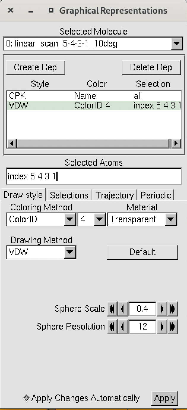
The numbering of the dihedral angles matches the VMD indexing, so the four atoms are selected in VMD as 5, 4, 3, and 1. You can see the selection in VMD below:
Now, we can finally plot the results of the scan using xmgrace or another plotting program, by plotting the data from the dat file.
For instance, using xmgrace, we can run the following command:
xmgrace linear_scan_5-4-3-1_30deg.dat
This will give us a plot of the energy vs dihedral angle, which should look something like this:
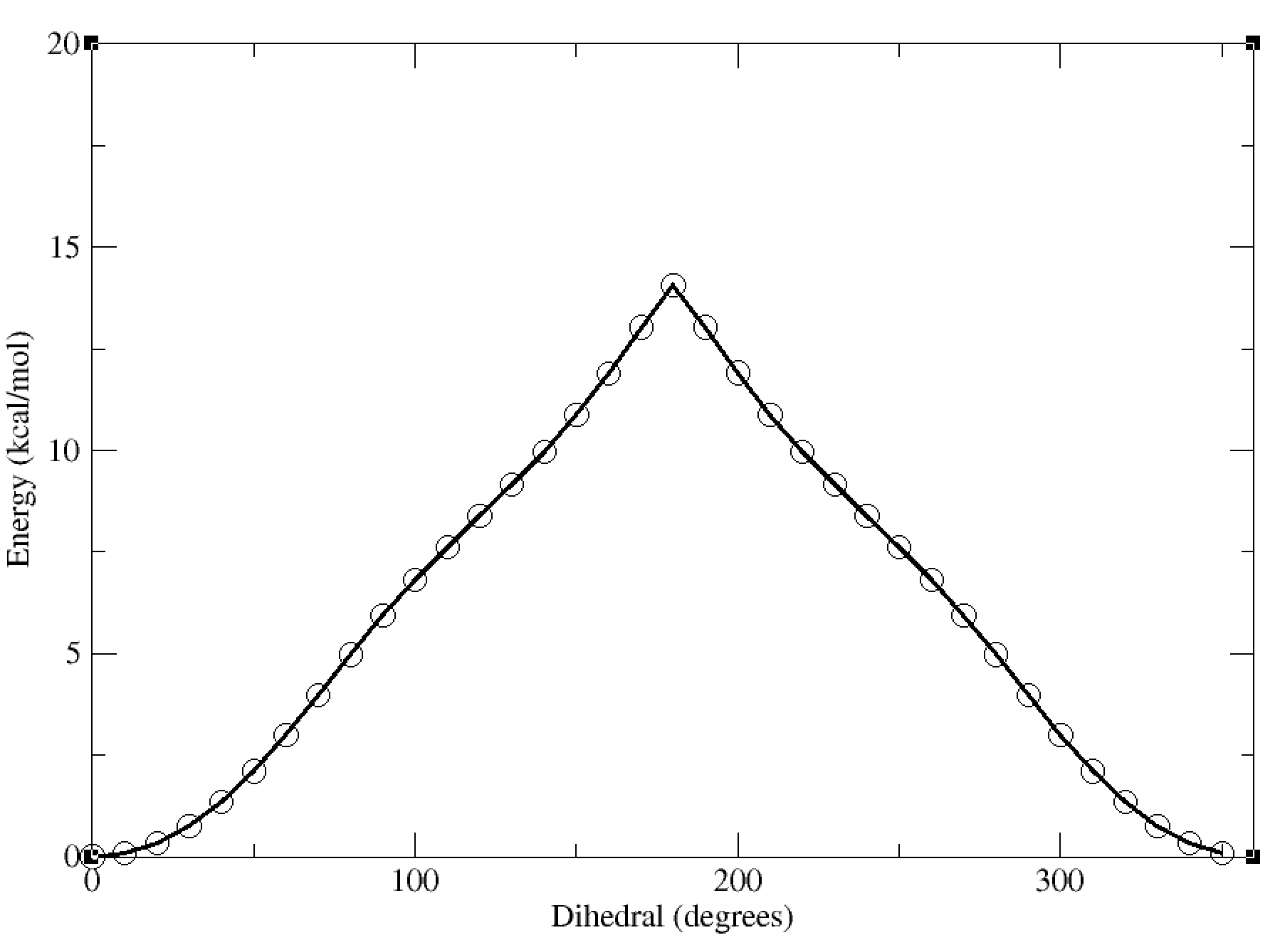
In this case, the dihedral angle is at a minimum at 0 degrees, which corresponds to the planar conformation of the amide. The energy increases as the dihedral angle deviates from this value, reaching a maximum at 180 degrees.
In this tutorial, we will be using a small molecular fragment that contains a deprotonated amide. These fragments can show up in certain ligands, and are presently a challenge for standard force field generation within amber. We will walk through how to use FFPOPT to scan dihedral angles with both MD force-fields and machine learning potentials, and then we will walk through the process of fitting new dihedral parameters.
The files you will need are located here:
WaveFront Dihedral Scans
Introduction to WaveFront Scans
In this section, we will be using the WaveFront scanning method to scan dihedral angles. The WaveFront method is a more effective way to scan dihedrals compared to traditional linear scans (which scan dihedrals sequentially). WaveFront scans work on the other hand by using a propagating wave approach, where dihedral scans begin from a certain set of “starting_nodes” (i.e., specific values of the dihedral angles). Each of these starting nodes are geometry optimized (with the value of the dihedral fixed), and an energy calculated. These nodes are then used to propagate new nodes in the next level of the WaveFront scan, which repeat the process. New nodes are only created if they either have not been calculated yet, or if the new node has a lower energy than a previously calculated node at that dihedral value. This process continues until all dihedral values have been scanned, and all nodes do not generate any new lower energy nodes.
Hint
Terminology:
Starting Nodes: The initial set of dihedral values to begin the scan from.
Nodes: Specific configurations of the molecule at given dihedral angles.
Levels: Each iteration of the scan where new nodes are generated from the previous level. Nodes within a level can be computed in parallel.
WaveFront: The overall scanning method that utilizes the above concepts to efficiently explore the dihedral space.
The key advantage of the WaveFront method is that it allows for significant parallelization of calculations, and in general, it also allows for significantly lower energy conformation to be found at each dihedral value, since geometries are propagated from multiple different directions.
The general logic is as follows:
Geometry optimize the molecule with no dihedral restraints
Choose a set of starting nodes (i.e., dihedral values to begin the scan from), and geometry optimize the molecule at each of these dihedral values (with the dihedral restrained)
For each starting node, generate new nodes by incrementing/decrementing the dihedral by the scan step size (e.g., if the starting node is at 0 degrees, and the step size is 15 degrees, new nodes would be generated at -15 and +15 degrees)
Run the second level, which are these new nodes, geometry optimizing each (with the dihedral restrained) and calculating the energy
If a new node is at a dihedral value that has not been calculated yet, add it to the list of calculated nodes. If it is at a dihedral value that has been calculated, only keep it if its energy is lower than the previously calculated node at that dihedral value.
Repeat steps 3-5 until all dihedral values have been scanned, and no new lower energy nodes are found.
The schematic below illustrates the WaveFront scanning method:
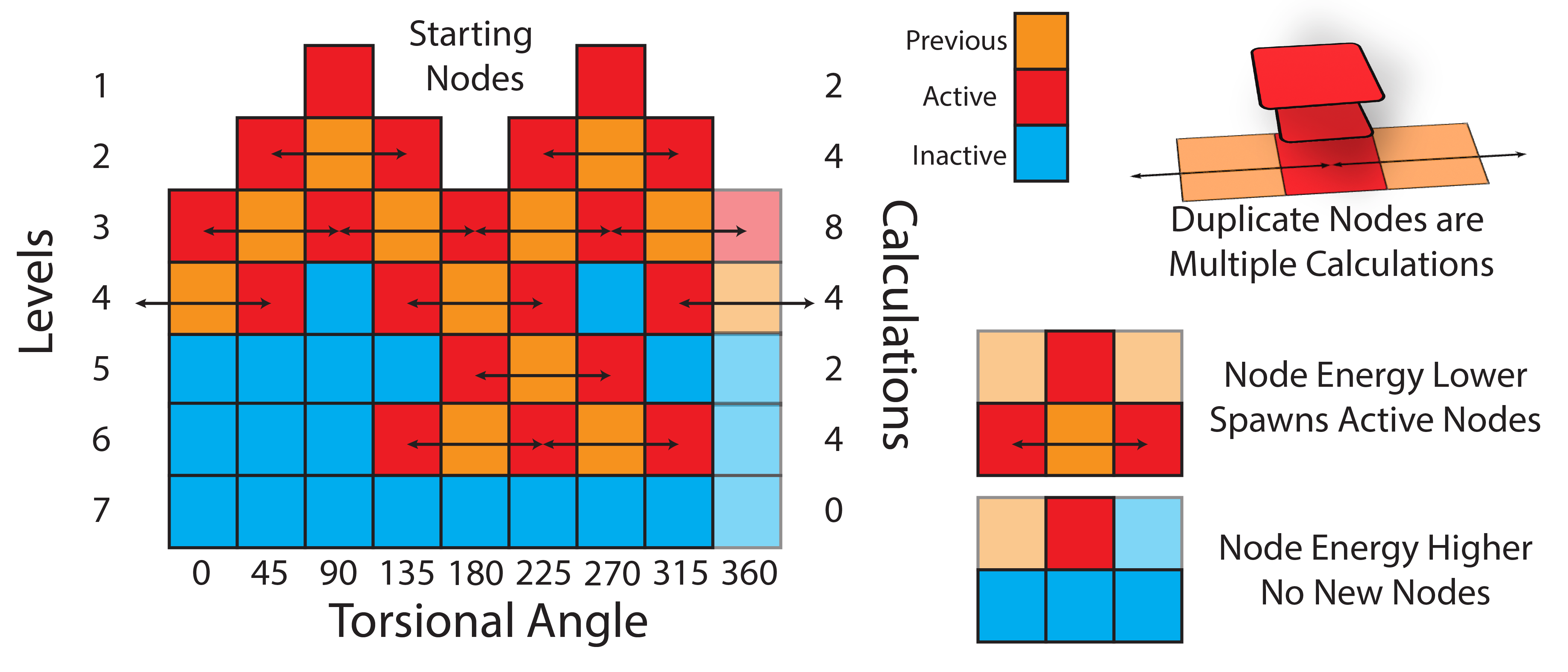
This often leads to many more total calculations; however, due to the parallelizability of each level of the scan, this is often significantly faster than a traditional linear scan, especially as computational methods become more expensive.
Scans on the mmm_NN Model System
In this tutorial, we will apply the WaveFront scanning method to the same model system used in the Linear Scan Tutorial. As a reminder, this molecule is a small fragment containing a deprotonated amide, which can be challenging for standard force field generation methods.
Using the provided input files, we will run WaveFront dihedral scans using the gaff2 force field, as well as a higher level machine learning potential, QDPi2, which has been developed within the York Group and is available in FFPOPT.
To get started, we will first run the most basic type of WaveFront scan on this system, which is a single dihedral scan using the gaff2 force field. As with the LinearScan Tutorial we will be scanning the 5-4-3-1 dihedral that links the nitrogen to the five-membered ring. See a movie of the molecule below:
In the movie, the dihedral being scanned is highlighted in yellow for clarity.
To run a WaveFrotn scan using FFPOPT, we will use the following command:
ffpopt-DihedWavefront.py -p mmm_NN.parm7 -c mmm_NN.rst7 --model=sander --dihed="5,4,3,1" --oscan wf_scan_5-4-3-1_s1_n0.xyz --delta 10 --nproc 10 --wf_starting_nodes 1 --wf_num_conformers 0
Here, note that the argument structure is very similar to the linear scan commands; however, there are some key differences to note:
nproc: This argument specifies the number of processors to use for the scan. Since WaveFront scans can be parallelized, this argument is important to set appropriately based on available computational resources.
wf_starting_nodes: This argument specifies the number of starting nodes to use for the WaveFront scan. In this case, we are using 1 starting node, which will be the optimized geometry without any dihedral restraints.
wf_num_conformers: This argument specifies the number of conformers to generate at each new node. Setting this to 0 means that no additional conformers will be generated, and only the geometry optimized at the dihedral restraint will be used.
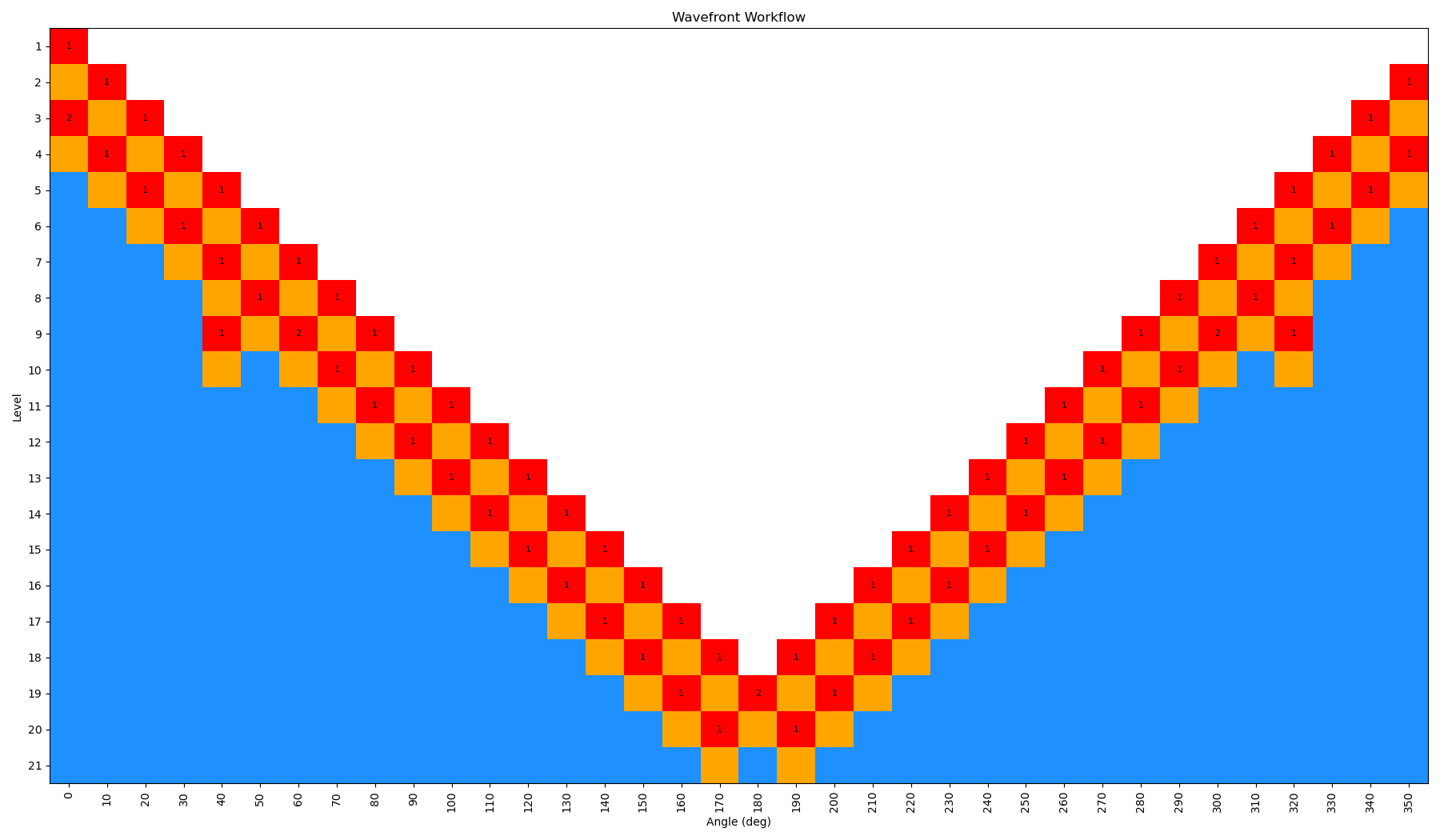
After this command is run, FFPOPT will output information to the terminal about the progress of the WaveFront scan, including the current level, how many nodes are being calculated, and the dihedral values of the nodes being processed.
When the scan is complete, the output file wf_scan_5-4-3-1_s1_n0.xyz will contain the results of the scan, including the optimized geometries and energies at each dihedral value, and as with before the energies are included in a output file called wf_scan_5-4-3-1_s1_n0.dat. In addition to these files, the scan also writes a pickled checkpoint file called checkpoint_wf_scan_5-4-3-1_s1_n0.pkl, which contains all of the information about the scan, including the geometries and energies of each node. This file can be used to restart the scan if needed, or to analyze the results further. Lastly, an image file called wf_workflow_wf_scan_5-4-3-1_s1_n0.png is also generated, which contains a schematic diagram of the levels and nodes of the WaveFront scan that were explored during the run.
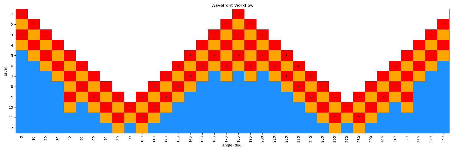
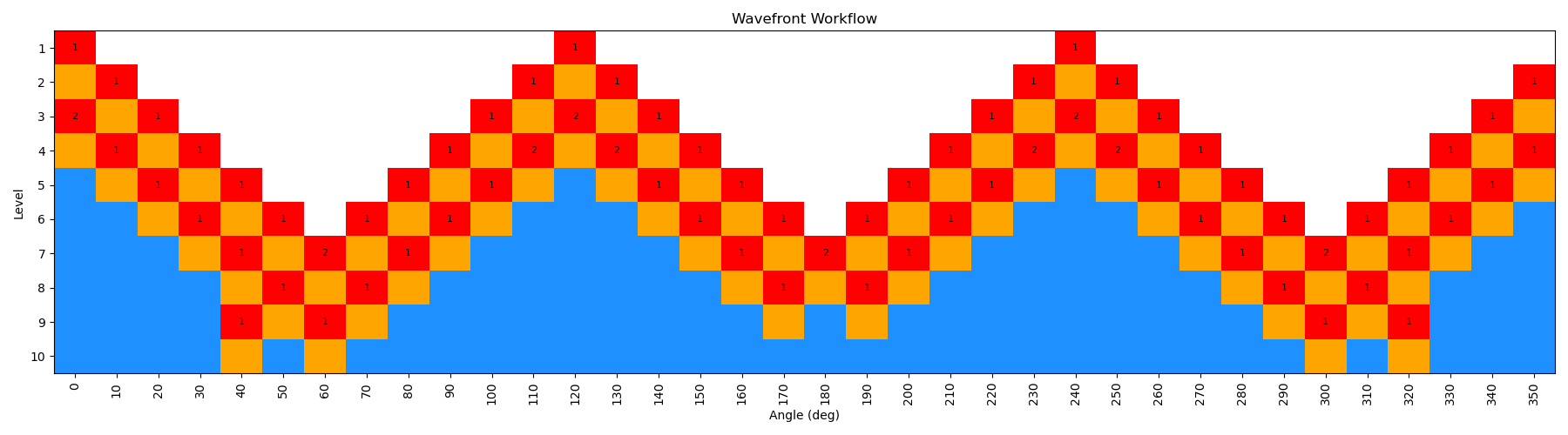
By incrementing the number of starting nodes (from 1 to 4), we can often improve the quality of the scan as more starting structures are propagated. For this particular molecule, there is not a huge difference with GAFF2; however, for more complex molecules this can be very important. In the below figure, we show both the code-block to run the scan with different starting nodes, as well as diagrams of the scan.
ffpopt-DihedWavefront.py -p mmm_NN.parm7 -c mmm_NN.rst7 --model=sander --dihed="5,4,3,1" --oscan wf_scan_5-4-3-1_s1_n0.xyz --delta 10 --nproc 10 --wf_starting_nodes 1 --wf_num_conformers 0
ffpopt-DihedWavefront.py -p mmm_NN.parm7 -c mmm_NN.rst7 --model=sander --dihed="5,4,3,1" --oscan wf_scan_5-4-3-1_s2_n0.xyz --delta 10 --nproc 10 --wf_starting_nodes 2 --wf_num_conformers 0
ffpopt-DihedWavefront.py -p mmm_NN.parm7 -c mmm_NN.rst7 --model=sander --dihed="5,4,3,1" --oscan wf_scan_5-4-3-1_s3_n0.xyz --delta 10 --nproc 10 --wf_starting_nodes 3 --wf_num_conformers 0
ffpopt-DihedWavefront.py -p mmm_NN.parm7 -c mmm_NN.rst7 --model=sander --dihed="5,4,3,1" --oscan wf_scan_5-4-3-1_s4_n0.xyz --delta 10 --nproc 10 --wf_starting_nodes 4 --wf_num_conformers 0
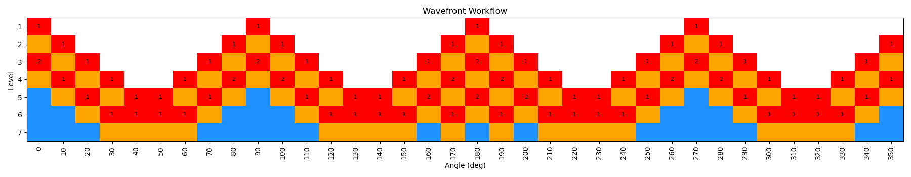
Note - that as the number of starting nodes increases, the number of levels in the wavefront calculation generally goes down (as more of the dihedral space is covered from the start), but the number of total nodes calculated generally goes up (as more nodes are propagated from each starting node). However, since each level can be parallelized, the overall wall time of the calculation can often go down with more starting nodes, especially at higher levels of theory.
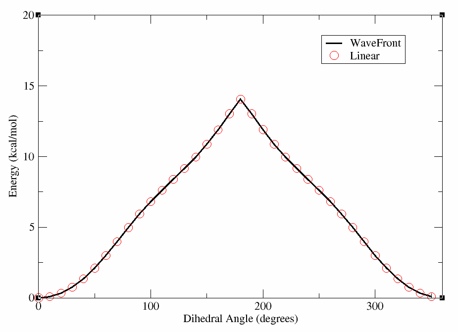
Now, we can make a plot of the energy vs. dihedral angle for each of these scans, and compare them to the linear scan done previously with GAFF2 using xmgrace (or a plotting program of your choice). In the figure below, we show the results of the WaveFront scans with different starting nodes, as well as the linear scan for comparison. We have included the linear scan data file for reference, though it can be produced in the Linear Scan Tutorial.
xmgrace wf_scan_5-4-3-1_s1_n0.dat wf_scan_linear.dat
This will produce a plot where the lines overlap nearly perfectly, indicating that for this molecule the WaveFront scan is producing similar results to the linear scan with GAFF2. We will show an example later where this is not the case; however, for clarity we have included the plot below.
Now, we can move on to running a WaveFront scan using a higher level of theory, specifically the QDPi2 machine learning potential. This potential has been trained on high-level quantum mechanical data at the SPICE level of theory, and can often provide more accurate results than traditional force fields like GAFF2. QDPI2 is a delta-Machine learning potential, meaning that it predicts the difference between a lower level of theory (XTB) and a higher level of theory (SPICE). Therefore, within FFPOPT, QDPI2 scans are run by first performing an XTB calculation, and then applying the QDPi2 correction to obtain the final energy. This is handled completely internally within FFPOPT, so the user does not need to worry about the details.
To run a WaveFront scan using QDPi2, we will use the following command:
ffpopt-DihedWavefront.py -p mmm_NN.parm7 -c mmm_NN.rst7 --model=qdpi2 --dihed="5,4,3,1" --oscan wf_scan_5-4-3-1_QDPi2_s4_n0.xyz --delta 10 --nproc 10 --wf_starting_nodes 4 --wf_num_conformers 0
You’ll notice straight away that the command is almost identical to the GAFF2 command, with the only difference being the model specified as “qdpi2” instead of “sander”. This is one of the key advantages of FFPOPT, as it allows for easy switching between different computational methods without changing the overall workflow.
Again, all the output files are more or less the same as before, with the main output being the optimized geometries and energies at each dihedral value in the wf_scan_5-4-3-1_QDPi2_s4_n0.xyz and wf_scan_5-4-3-1_QDPi2_s4_n0.dat files, respectively. A checkpoint file and workflow diagram are also generated as before. We use 4 starting nodes in the example here to ensure good coverage of the dihedral space.
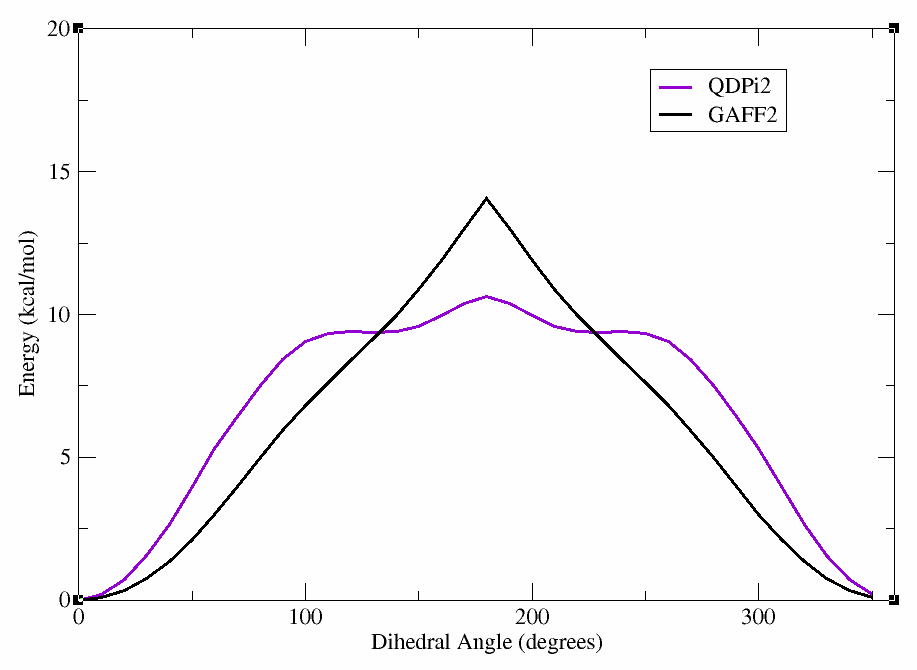
After the scan is complete, we can again plot the energy vs. dihedral angle using xmgrace (or a plotting program of your choice). In the figure below, we show the results of the QDPi2 WaveFront scan along with the previous GAFF2 scan for comparison.
xmgrace wf_scan_5-4-3-1_QDPi2_s4_n0.dat wf_scan_5-4-3-1_s4_n0.dat
This will produce a plot showing the differences between the GAFF2 and QDPi2 scans. As can be seen, there are significant differences in the energy profiles, particularly around certain dihedral angles. This highlights the importance of using higher-level methods for accurate dihedral parameterization.
Hint
If you kill a wavefront scan before it is complete, it writes a checkpoint for each node, level, and the whole calculation. It will try to use these to restart the calculation when you run the same command again. If you want to start fresh, delete the checkpoint files!
Another Example: Linear Scans Overestimate Barriers
In the previous example, we saw that the WaveFront and Linear scans with GAFF2 produced similar results for the mmm_NN molecule. However, this is not always the case, especially for more complex molecules or those with multiple rotatable bonds. To illustrate this, we will consider another molecule, which we will refer to as “complex_mol”. This molecule has multiple rotatable bonds and a more complex conformational landscape, making it a good candidate for demonstrating the advantages of the WaveFront scanning method.
This molecule has the same dihedral as before, involving a deprotonated amide going into a five-membered ring. Try loading the molecule into VMD to identify the atoms involved in the dihedral.
Hint
In VMD, you can load the provided binder.parm7 and binder.rst7 files to visualize the molecule and identify the dihedral of interest.
vmd binder.parm7 binder.rst7
In VMD, you can click the 4 key to go into dihedral selection mode, and then select the four atoms of the dihedral. Select the C - N - C - S atoms. You should see the dihedral is close to zero (-2.6 degrees).
In the terminal, you can see that these atoms correspond to atoms 15-5-1-2 by looking at the index entry for each atom.
Now we will run the WaveFront scan on this molecule using GAFF2, similar to before. We will use 4 starting nodes to ensure good coverage of the dihedral space. The command is as follows:
ffpopt-DihedWavefront.py -p binder.parm7 -c binder.rst7 --model=sander --dihed="15,5,1,2" --oscan wf_scan_binder_15-5-1-2_s4_n0.xyz --delta 10 --nproc 10 --wf_starting_nodes 4 --wf_num_conformers 0
Note
This molecule is more complex, and much larger than the previous example, so the scan may take significantly longer to complete!
Warning
Sometimes the WaveFront scan may take an inoordinate amount of time on complex molecules due to bad overlaps in the propagated geometries. If this happens, you can try changing the number of starting nodes to avoid generating a clash. Alternatively, you can try running with the ase-optimizer instead of GEOMETRIC, which sometimes performs better in these cases.
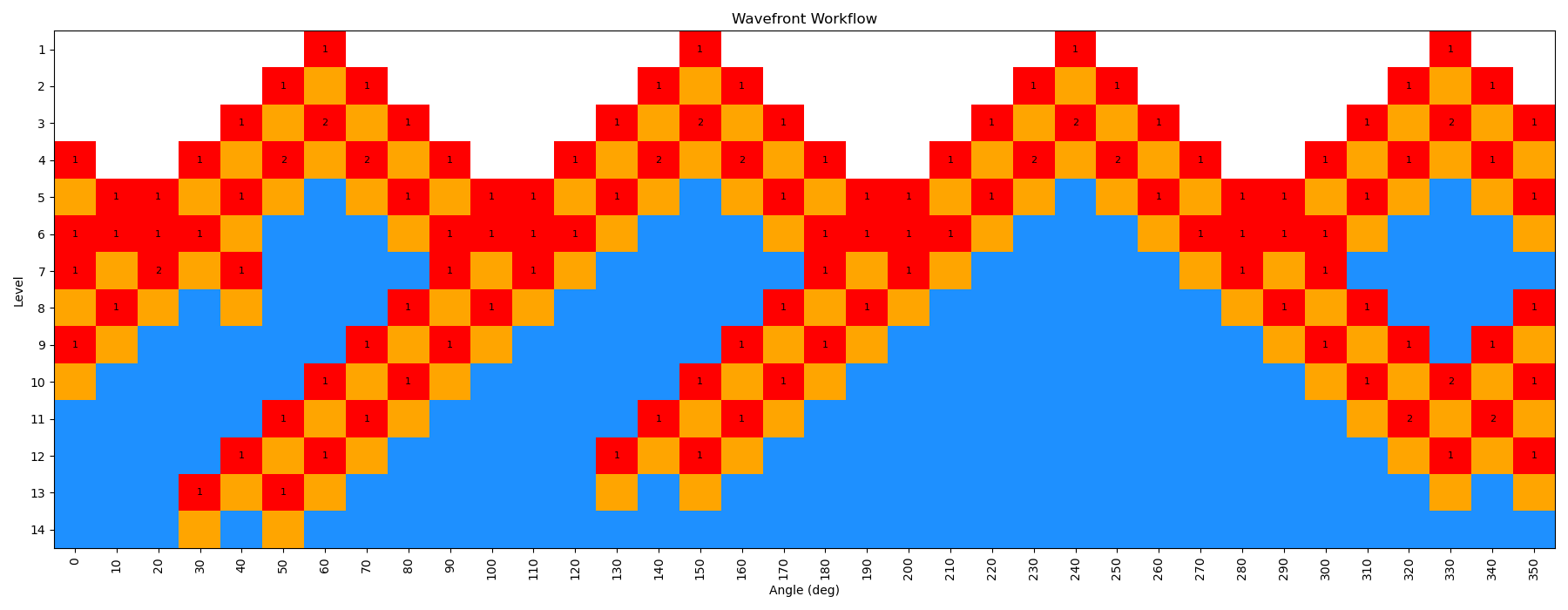
This scan is actually a bit more interesting than the previous example, as the WaveFront scan revisits a number of geometries it had already calculated, indicating that it was able to find a lower energy conformation at those dihedral values. This is one of the key advantages of the method, as it allows for a more thorough exploration of the conformational space.
You can see that here in this figure:
We have repeated the wavefront scan using QDPi2 as well, using the following command:
ffpopt-DihedWavefront.py -p binder.parm7 -c binder.rst7 --model=qdpi2 --dihed="15,5,1,2" --oscan wf_scan_binder_15-5-1-2_QDPi2_s4_n0.xyz --delta 10 --nproc 10 --wf_starting_nodes 4 --wf_num_conformers 0
Warning
The QDPI2 scan likely takes more time than you want to do, especially without a gpu. If you want to skip this step, you can move on to the analysis section below.
After both scans are complete, we can plot the energy vs. dihedral angle for both GAFF2 and QDPi2 using xmgrace (or a plotting program of your choice). In the figure below, we show the results of both scans.
xmgrace wf_scan_binder_15-5-1-2_s4_n0.dat wf_scan_binder_15-5-1-2_QDPi2_s4_n0.dat
In this tutorial, we will be using a small molecular fragment that contains a deprotonated amide. These fragments can show up in certain ligands, and are presently a challenge for standard force field generation within amber. We will walk through how to use FFPOPT to scan dihedral angles with both MD force-fields and machine learning potentials, and then we will walk through the process of fitting new dihedral parameters.
The files you will need are located here:
Dihedral Fitting
Often, when parameterizing a new molecule for a molecular dynamics simulation, the default force field parameters will not accurately capture the torsional energy landscape of certain dihedral angles. In these cases, it is necessary to fit new dihedral parameters to better reproduce high-level quantum mechanical calculations or machine learning potential energy surfaces.
In this tutorial, we will use FFPOPT to fit new dihedral parameters for the deprotonated amide fragment for the GAFF2 force-field, using the QDPI2 machine learning potential as our reference “high-level” method.
Roughly, FFPOPT approaches dihedral fitting in the following way:
Perform a conformational scan of the dihedral(s) of interest using both the existing force field and the reference method (here, QDPI2).
Compare the energy profiles from the force field and the reference method.
Generate primative dihedrals that can be used to fit the difference between the two energy profiles.
Re-calculate the energy profile using the modified force field with the new dihedral parameters.
Iterate the fitting process until the force field energy profile closely matches the reference method.
To get started with this, we will use the Dihedral Twist Workflow, which automates much of this process.
ffpopt-DihedTwistWorkflow.py --parm mmm_NN.parm7 --rst mmm_NN.rst7 --bond "4,3" --delta 10 --nprim 3 --nproc 10 --wf_starting_nodes 4 --geometric-converge 'set GAU' --model qdpi2 > scan.sh
This command will generate a script called scan.sh that contains all the necessary steps to perform the dihedral fitting workflow. You can then run this script to carry out the fitting process. If you explore the scan.sh file, you will see that it contains commands to perform the scans, generate the primative dihedrals, and fit the new parameters.
Opening up the scan.sh file, you will see commands calling the wavefront workflow to perform scans at both they low and high levels of theory, as well as commands to generate new dihedral parameters and run scans on those iteratively until new parameters are reached.
Note
The script, ffpopt-DihedTwistWorkflow.py, has many options that can be adjusted to fit your specific needs, and accepts any arguments that the WaveFront method accepts. You can explore these options by running ffpopt-DihedTwistWorkflow.py –help.
Taking a look at scan.sh, you will see that it contains commands calling the wavefront workflow to perform scans at both they low and high levels of theory, as well as commands to generate new dihedral parameters and run scans on those iteratively until new parameters are reached.
Take a look at the file below that is generated. You’ll see that it contains calls to the wavefront method to perform scans at both the low and high levels of theory, as well as calls to generate new dihedral parameters and run scans on those iteratively until new parameters are reached.
#!/bin/bash
set -e
set -u

# High level scan with QDPi2
if [ ! -e qdpi2_5-4-3-1.xyz ]; then
    echo Creating qdpi2_5-4-3-1.xyz
    ffpopt-DihedWavefront.py -p mmm_NN.parm7 -c mmm_NN.rst7 --model qdpi2 --dihed="5,4,3,1" \
        --oscan qdpi2_5-4-3-1.xyz --delta 10 --nproc 1 --wf_starting_nodes 4 --wf_max_levels -1 --wf_num_conformers 0 --geometric-converge 'set GAU'

fi

# Low level scan with sander
if [ ! -e orig_5-4-3-1.xyz ]; then
    echo Creating orig_5-4-3-1.xyz
    ffpopt-DihedWavefront.py -p mmm_NN.parm7 -c mmm_NN.rst7 --model=sander --dihed="5,4,3,1" \
        --oscan orig_5-4-3-1.xyz --delta 10 --nproc 1 --wf_starting_nodes 4 --wf_max_levels -1 --wf_num_conformers 0 --geometric-converge 'set GAU'

fi

# Iteration 1 Fitting
if [ ! -e it01.py ]; then
    echo Creating it01.py
    ffpopt-GenDihedFit.py --nlmaxiter=300  --ase-opt it01.json
fi

# Make new parm7 with it01.py
if [ ! -e it01.parm7 ]; then
    echo Creating it01.parm7
    python3 it01.py mmm_NN.parm7 it01.parm7
fi


# Calculate updated low level scan with it01.parm7
if [ ! -e it01_5-4-3-1.xyz ]; then
    echo Creating it01_5-4-3-1.xyz
    ffpopt-DihedWavefront.py -p it01.parm7 -c mmm_NN.rst7 --model sander --dihed="5,4,3,1" \
        --oscan it01_5-4-3-1.xyz --delta 10 --nproc 1 --wf_starting_nodes 4 --wf_max_levels -1 --wf_num_conformers 0 --geometric-converge 'set GAU'

fi

# Iteration 2 Fitting
if [ ! -e it02.py ]; then
    echo Creating it02.py
    ffpopt-GenDihedFit.py --nlmaxiter=300  --ase-opt it02.json
fi

# Make new parm7 with it02.py
if [ ! -e it02.parm7 ]; then
    echo Creating it02.parm7
    python3 it02.py mmm_NN.parm7 it02.parm7
fi

# Calculate updated low level scan with it02.parm7
if [ ! -e it02_5-4-3-1.xyz ]; then
    echo Creating it02_5-4-3-1.xyz
    ffpopt-DihedWavefront.py -p it02.parm7 -c mmm_NN.rst7 --model sander --dihed="5,4,3,1" \
        --oscan it02_5-4-3-1.xyz --delta 10 --nproc 1 --wf_starting_nodes 4 --wf_max_levels -1 --wf_num_conformers 0 --geometric-converge 'set GAU'

fi
We can then run this script to carry out the fitting process:
bash scan.sh
This will most likely take a while, depending on your computational resources. Once it is complete, you will have new dihedral parameters that better reproduce the QDPI2 energy profile for the dihedral of interest.
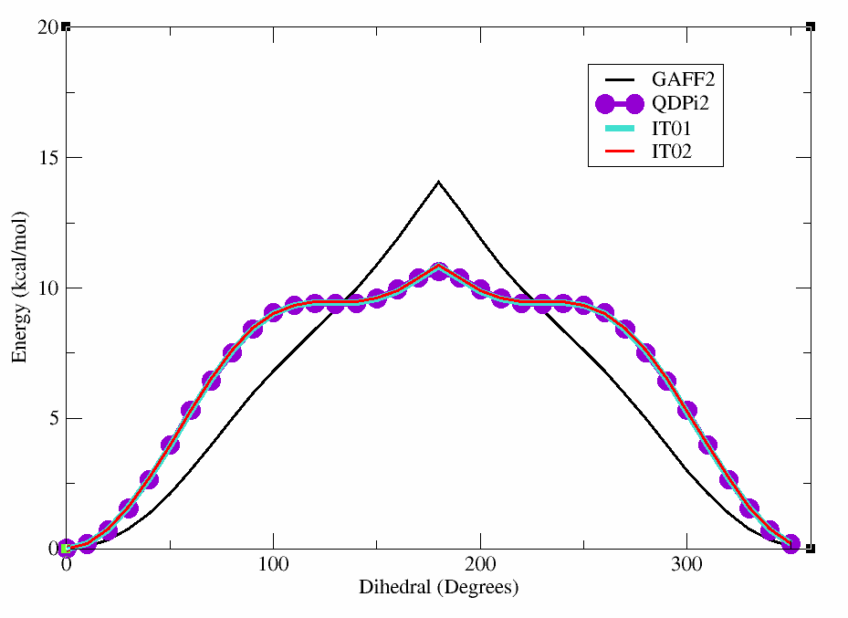
We can plot these results to see how well the new parameters reproduce the reference energy profile.
xmgrace orig_5-4-3-1.xyz qdpi2_5-4-3-1.xyz it01_5-4-3-1.xyz it02_5-4-3-1.xyz
You can see the plot below which shows the original GAFF2 parameters in black, the QDPI2 reference in purple,