11. Hands-On Session 11: Transfer learning: active learning to fine-tune a foundational machine learning potential to a specific target system for improved accuracy
11.1. Learning Objectives
Generate training data for a ΔMLP from AMBER simulation data
Write json style input files for training models with DeePMD-kit
Verify the setup by briefly training a model a producing the loss output
Use dptest to assess the accuracy of your model compared to a model after longer training
Demonstrate that the free energy profile obtained from ΔMLP simulatins of MTR1 is more accurate than DFTB3
11.2. Relevant literature
11.3. Activities
11.3.1. Workflow
        flowchart LR

%% ===== generate training data =====
A1["Input files<br/>qmmm.parm7<br/>it021/img001.nc<br/>img001.rst7"]
P1{{"<b>[§11.3.2]</b><br/>QM/MM single points<br/>then extract corrections<br/>sander.MPI / dpamber corr"}}
O1["<b>[from §11.3.2]</b><br/>Training dataset<br/>img001_DFTB3.hdf5"]
A1 --> P1
P1 --> O1

%% ===== generate DeePMD-Kit inputs =====
P2{{"<b>[§11.3.3]</b><br/>Write training and<br/>machine input files<br/>DeePMD-Kit"}}
O2["<b>[from §11.3.3]</b><br/>DeePMD-Kit configs<br/>simplify_MACE.json<br/>machine_simplify.json"]
O1 --> P2
P2 --> O2

%% ===== train a model =====
P3{{"<b>[§11.3.4]</b><br/>Train MACE model<br/>dpgen simplify / dp train"}}
O3["<b>[from §11.3.4]</b><br/>Trained model<br/>graph.000.pth<br/>lcurve.out"]
O2 --> P3
P3 --> O3

%% ===== validate the model =====
P4{{"<b>[§11.3.5]</b><br/>Validate on train and<br/>test sets<br/>dp test"}}
O4["<b>[from §11.3.5]</b><br/>Parity metrics<br/>parity_TrainingSet.out<br/>parity_TestSet.out"]
O3 --> P4
P4 --> O4

%% ===== apply transfer learning =====
A5["Foundational model<br/>Foundation_model/00.train"]
P5{{"<b>[§11.3.6]</b><br/>Refine from foundation<br/>model via transfer learning<br/>dpgen simplify"}}
O5["<b>[from §11.3.6]</b><br/>Refined model<br/>graph.000.pth"]
O3 --> P5
A5 --> P5
P5 --> O5

%% ===== model-deviation active learning =====
P6{{"<b>[§11.3.7]</b><br/>Compute force deviation<br/>over a committee<br/>dp model-devi"}}
O6["<b>[from §11.3.7]</b><br/>Model deviation<br/>model-devi_SRP.out<br/>model-devi_Refine.out"]
O5 --> P6
P6 --> O6

%% ===== on-the-fly active learning =====
P7{{"<b>[§11.3.8]</b><br/>On-the-fly active learning<br/>dpgen run"}}
O7["<b>[from §11.3.8]</b><br/>Updated committee model<br/>graph.00x.pth"]
O6 --> P7
P7 --> O7

classDef file fill:#fff7e6,stroke:#d98c00,stroke-width:1.5px,color:#111;
classDef program fill:#e8f1ff,stroke:#1f77b4,stroke-width:1.8px,color:#111;
classDef result fill:#eaf7ea,stroke:#2ca02c,stroke-width:1.5px,color:#111;
class A1,A5 file;
class P1,P2,P3,P4,P5,P6,P7 program;
class O1,O2,O3,O4,O5,O6,O7 result;
Download the necessary inputs for this activity:
Attention
Copy the directory to your working directory
cp -r /PATH2Files/HandsOn11-Train_inputs.tar.gz ./
tar -xzvf HandsOn11-Train_inputs.tar.gz
cd HandsOn11-Train_inputs
In this activity you will learn how to prepare QM/MM training data, train a QM/MM+ΔMLP model with DeePMD-Kit, then validate the accuracy of the model. The preparation is agnostic to the type of model you wish to train, so the data could be used to train a Deep Potential (DP) or Graph Neural Network (GNN) model. We will assume the low level, semi-empirical model is DFTB3, and the high level, ab initio target model is PBE0/6-31G*. In this activity we will train a MACE graph neural network potential. Specificaly, we will refine a foundational ΔMACE model pre-trained for nucleic acid enzyme reactions using transfer learning. The first step will be to prepare the training data which includes the positions of atoms within 6 angstroms of the QM region, otherwise known as the environment, and their associated forces and energies at the DFTB3 and PBE0 level. The model will be trained to correct the difference between the models.
11.3.2. Generate training data from AMBER QM/MM simulaitons
You will first need to peform umbrella sampling simulations to obtain the minimum free energy path using the low level potential. If your reaction is 1-dimensional, this is simply a linear interpolation from reactants to products; however, if your reaction contains multiple reaction coordinates, you must optimize the path using a string method. For this activity, we will use the 2-dimensional MTR1 MFEP obtained in Hands on session 5. For the sake of this activity, we will only perform training for a single umbrella window with a minimal number of training steps in order to obtain a model within the workshop time constraints. However, one could follow this procedure for all windows and increase the number of training steps for a real-world application.
25 ps of production sampling on the minimum free energy path have been performed for you. We will use the first umbrella window as an example for this exercise. In order to generate training data, we will perform single point calculations using the DFTB3 and PBE0 methods to output the forces and energies to .mdfrc and .mden file, respectively. The trajectory is recommended to contain 100 frames, but you will perform single point calculations for only the first two frames for time purposes. Download the inputs and navigate to the HandsOn11-Train_inputs directory:
cd HandsOn11-Train_inputs/GenData
ls
TEMPLATE_DFTB3.mdin  TEMPLATE_PBE0.mdin  it021  reanalyze_array.slurm  slurm  template

ls it021
img001.disang  img001.nc  img001.rst7
The necessary outputs from production are contained in it021. You have been provided two input files for single point calculations, one with DFTB3 and one with PBE0.
DFTB3
&cntrl
! IO =======================================
      irest = 0       ! 0 = start, 1 = restart
      ntx = 1       ! 1 = start, 5 = restart
      ntxo = 1       ! read/write rst as formatted file
      iwrap = 1       ! wrap crds to unit cell
      ioutfm = 1       ! write mdcrd as netcdf
      imin = 6
      ntmin = 1
      ntpr = 1
      ntwr = 0
      ntwx = 0
      ntwf = 1       ! print mdfrc file
      ntwe = 1       ! print mdene file
! DYNAMICS =================================
    nstlim = 0    ! number of time steps
        dt = 0.001   ! ps/step
        ntb = 1       ! 1=NVT periodic, 2=NPT periodic, 0=no box
! TEMPERATURE ==============================
      temp0 = 298     ! target temp
  gamma_ln = 5.0     ! Langevin collision freq
        ntt = 3       ! thermostat (3=Langevin)
! PRESSURE  ================================
        ntp = 0       ! 0=no scaling, 1=isotropic, 2=anisotropic
! SHAKE ====================================
        ntc = 2       ! 1=no shake, 2=HX constrained, 3=all constrained
noshakemask = ":69|@272-282,290-291,1975-1988"    ! do not shake these
        ntf = 1       ! 1=cpt all bond E, 2=ignore HX bond E, 3=ignore all bond E
! MISC =====================================
        cut = 10.0
      ifqnt = 1
        ig = -1
    nmropt = 0
    lj1264 = 0
/


&ewald
  dsum_tol = 1.e-6
/

&qmmm
    qm_theory   = 'DFTB3'
        qmmask  = ':69|@272-282,290-291,1975-1988'
      qmcharge  = 1
          spin  = 1
      qmshake  = 0
      qm_ewald  = 1
  qmmm_switch  = 1
      scfconv  = 1.e-10
    verbosity  = 0
  tight_p_conv  = 1
  diag_routine  = 0
  pseudo_diag  = 1
  dftb_maxiter  = 100
/

&wt type = 'DUMPFREQ', istep1 = 8, /
&wt type='END' /
DISANG=imgXXXX.disang
DUMPAVE=imgXXXX.dumpave
LISTOUT=POUT
LISTIN=POUT
PBE0
&cntrl
! IO =======================================
      irest = 0       ! 0 = start, 1 = restart
      ntx = 1       ! 1 = start, 5 = restart
      ntxo = 1       ! read/write rst as formatted file
      iwrap = 1       ! wrap crds to unit cell
      ioutfm = 1       ! write mdcrd as netcdf
      imin = 6
      ntmin = 1
      ntpr = 1
      ntwr = 0
      ntwx = 0
      ntwf = 1
      ntwe = 1
! DYNAMICS =================================
    nstlim = 0    ! number of time steps
        dt = 0.001   ! ps/step
        ntb = 1       ! 1=NVT periodic, 2=NPT periodic, 0=no box
! TEMPERATURE ==============================
      temp0 = 298     ! target temp
  gamma_ln = 5.0     ! Langevin collision freq
        ntt = 3       ! thermostat (3=Langevin)
! PRESSURE  ================================
        ntp = 0       ! 0=no scaling, 1=isotropic, 2=anisotropic
! SHAKE ====================================
        ntc = 2       ! 1=no shake, 2=HX constrained, 3=all constrained
noshakemask = ":69|@272-282,290-291,1975-1988"    ! do not shake these
        ntf = 1       ! 1=cpt all bond E, 2=ignore HX bond E, 3=ignore all bond E
! MISC =====================================
        cut = 10.0
      ifqnt = 1
        ig = -1
    nmropt = 0
/


&ewald
  dsum_tol = 1.e-6
/

&qmmm
    qm_theory   = 'quick'
        qmmask  = ':69|@272-282,290-291,1975-1988'
      qmcharge  = 1
          spin  = 1
      qmmm_int  = 1
      qm_ewald  = 1
      qmshake  = 0
        itrmax  = 50
      scfconv  = 1e-07
    verbosity  = 0
/

&quick
  method   = 'PBE0'
  basis    = '6-31G*'
/

&wt type = 'DUMPFREQ', istep1 = 25, /
&wt type='END' /
DISANG=imgXXXX.disang
DUMPAVE=imgXXXX.dumpave
LISTOUT=POUT
LISTIN=POUT
Note that imin is set to 6 and nstlim is set to 0 for reanalysis. We will use QUICK to perform the high level calculations. Now take a look at reanalyze_array.slurm:
#!/bin/bash
#SBATCH --job-name="reanalysis_4Training"
#SBATCH --output="slurm/reanalysis_%a.slurmout"
#SBATCH --error="slurm/reanalysis_%a.slurmerr"
#SBATCH --partition={{CPUpartition}}
#SBATCH --nodes=1
#SBATCH --ntasks=16
#SBATCH --cpus-per-task=1
#SBATCH --mem=60G
#SBATCH --export=ALL
#SBATCH -t 0-00:30:00
#SBATCH --array=0       ##### Use for running 1st window
##SBATCH --array=0-31   ##### Use for running all windows


{{amberload}}

export QUICK_BASIS=${AMBERHOME}/AmberTools/src/quick/basis

qmreg=':69|@272-282,290-291,1975-1988'

top=`pwd`

i=021

RC=($(seq -w 1 1 32))            ##### If running all windows, img number is taken from the SLURM_ARRAY_TASK_ID
R=0${RC[${SLURM_ARRAY_TASK_ID}]}
echo R is ${R}

cd it${i}
if [ ! -d reanalysis ]; then mkdir reanalysis; fi
cd reanalysis

BASE=img${R}
PBE0=img${R}_PBE0
DFTB=img${R}_DFTB3
parm=qmmm.parm7

sed -e "s/XXXX/${R}/g" ${top}/TEMPLATE_DFTB3.mdin > img${R}_DFTB3.mdin
sed -e "s/XXXX/${R}/g" ${top}/TEMPLATE_PBE0.mdin > img${R}_PBE0.mdin

time mpirun -n 16 sander.MPI -O -p ../../template/${parm} -i ${DFTB}.mdin -c ../${BASE}.rst7 -o ene_${DFTB}.mdout -y ../${BASE}.nc -frc ene_${DFTB}.mdfrc -e ene_${DFTB}.mden -inf ${DFTB}.mdinfo

time mpirun -n 16 sander.MPI -O -p ../../template/${parm} -i ${PBE0}.mdin -c ../${BASE}.rst7 -o ene_${PBE0}.mdout -y ../${BASE}.nc -frc ene_${PBE0}.mdfrc -e ene_${PBE0}.mden -inf ${PBE0}.mdinfo


if [[ $(grep -r "TIMINGS" ene_${DFTB}.mdout) ]] && [[ $(grep -r "TIMINGS" ene_${PBE0}.mdout) ]]; then
  echo "${BASE} finished correctly"

  module purge
  {{dpgenload}}
  export OMP_NUM_THREADS=1
  export TF_INTER_OP_PARALLELISM_THREADS=1
  export TF_INTRA_OP_PARALLELISM_THREADS=1

  hl=ene_img${R}_PBE0
  ll=ene_img${R}_DFTB3
  out=img${R}_DFTB3.hdf5
  nc=../img${R}.nc
  dpamber corr --cutoff 6. --qm_region ${qmreg} --parm7_file ${top}/template/qmmm.parm7 --nc ${nc} --hl ${hl} --ll ${ll} --out ${out}

else
  exit 1
fi
Note that this slurm script is structured as a slurm array, so it can be easily be scaled for all umbrella windows by setting #SBATCH –array=0-31. For a sinlge window we just set it to 0. First, the script will write mdin files from the TEMPLATE files above. Then it will read in it021/img001.nc and perform single points at the DFTB3 and PBE0 levels. You must provide -frc and -mden flags here, along with setting ntwf and ntwe equal to 1 in the mdin file to output forces and energies. Finally, we will use the dpamber corr functionality from DeePMD-kit to extract necessary data from our outputs and package it in hdf5 file format. This is a pickle file that can be easily read by python. Specifically, the environment, ie coordinates of atoms within rcut and their associated elements, will be extracted from the trajectory. The associated differences in forces and energies will also be extracted.
The job should take approximately 10 minutes. Submit the job:
sbatch reanalyze_array.slurm
There should be a reanalysis directory created within it021. Navigate to the directory:
cd it021/reanalysis
The DFTB3 outputs should appear quickly once the jobs begins. When the job is complete, the img001_DFTB3.hdf5 should be produced:
ls
ene_img001_DFTB3.mden   ene_img001_DFTB3.mdout  ene_img001_PBE0.mdfrc  img001_DFTB3.hdf5  img001_DFTB3.mdinfo  img001_PBE0.mdinfo
ene_img001_DFTB3.mdfrc  ene_img001_PBE0.mden    ene_img001_PBE0.mdout  img001_DFTB3.mdin  img001_PBE0.mdin     quick.out
Let’s inspect the contents of img001_DFTB3.hdf5:
h5ls img001_DFTB3.hdf5
C15H16HW94N13O2OW49mC83mCl0mH94mN36mNa6mO48mP7 Group
C15H16HW95N13O2OW50mC83mCl0mH92mN37mNa6mO48mP6 Group

h5ls img001_DFTB3.hdf5/C15H16HW94N13O2OW49mC83mCl0mH94mN36mNa6mO48mP7
nopbc                    Dataset {SCALAR}
set.000                  Group
type.raw                 Dataset {463}
type_map.raw             Dataset {13}

h5ls img001_DFTB3.hdf5/C15H16HW94N13O2OW49mC83mCl0mH94mN36mNa6mO48mP7/set.000
aparam.npy               Dataset {1, 463}
coord.npy                Dataset {1, 1389}
energy.npy               Dataset {1}
force.npy                Dataset {1, 1389}
Each unique environment, or combination of atoms within rcut, is assigned to a group labeled by the element and number of occurances of the element in that structure. MM atoms have an “m” preceeding the element. Here we only have two structures. Looking further into the first entry, it contains information related to whether the system has periodic boundary conditions (nopbc), the data set (set.000), the elements types for every atom (type.raw), and the unique element types (type_map.raw). The number in {} indicates the length of the array. Looking further into set.000, we see that this is where the forces, energies, and coordinates are stored. There is also an entry called aparam indicating which residue the atoms belong to.
You have been provided the full data file for all of the frames. You can verify that the data you obtained matches is contained within that full data set:
The outputs can be downloaded here:
Attention
11.3.3. Generating input files for a DeePMD-Kit
The input files for DeePMD-kit training are in .json or .yaml format. These are structured like a dictionary in python. There is one input file providing the training and hyperparameters (simplfy_MACE.json), and another specifying the computational resources that will ultimately be used to write a slurm script (machine_simplify.json). You have been provided all of the necessary inputs for training.
cd HandsOn11-Train_inputs/Train/SRP
ls
common  computerprofiles simplify_MACE.json

ls computerprofiles
machine_simplify.json

ls common
img001_DFTB3.hdf5
The img001_DFTB3.hdf5 file produced in the previous step has been placed in the common directory. Let’s take a look at simplify_MACE.json:
{
  "default_training_param": {
    "model": {
      "type": "mace",
      "type_map": ["C","H","N","O","P","Mg","Ca","Na","Zn","S","HW","OW","mC","mCl","mH","mMg","mN","mNa","mO","mP","mS"],
      "r_max": 6.0,
      "sel": 128,
      "num_radial_basis": 8,
      "num_cutoff_basis": 5,
      "max_ell": 3,
      "interaction": "RealAgnosticResidualInteractionBlock",
      "num_interactions": 2,
      "hidden_irreps": "128x0e + 128x1o",
      "pair_repulsion": false,
      "distance_transform": "None",
      "correlation": 3,
      "gate": "silu",
      "MLP_irreps": "16x0e",
      "radial_type": "bessel",
      "radial_MLP": [
        64,
        64,
        64
      ]
    },
    "learning_rate": {
      "type": "exp",
      "start_lr": 0.001,
      "decay_steps": 2000,
      "stop_lr": 1e-05
    },
    "loss": {
      "type": "ener",
      "start_pref_e": 1,
      "limit_pref_e": 100,
      "start_pref_f": 100,
      "limit_pref_f": 100,
      "start_pref_v": 0,
      "limit_pref_v": 0
    },
    "training": {
      "numb_steps": 2000,
      "disp_file": "lcurve.out",
      "disp_freq": 100,
      "save_freq": 1000,
      "disp_training": true,
      "time_training": true,
      "profiling": false,
      "profiling_file": "timeline.json"
    }
  },
  "type_map": ["C","H","N","O","P","Mg","Ca","Na","Zn","S","HW","OW","mC","mCl","mH","mMg","mN","mNa","mO","mP","mS"],
  "pick_data": "common/img001_DFTB3.hdf5",
  "sys_configs": [],
  "sys_batch_size": ["auto"],
  "init_pick_number": 20000,
  "iter_pick_number": 10000,
  "numb_models": 1,
  "training_reuse_iter": 2,
  "training_reuse_start_lr": 0.001,
  "training_reuse_old_ratio": "auto",
  "training_reuse_numb_steps": 100000,
  "training_reuse_start_pref_e": 1,
  "training_reuse_start_pref_f": 100,
  "dp_compress": false,
  "model_devi_f_trust_lo": 0.08,
  "model_devi_f_trust_hi": 2.0,
  "labeled": true,
  "init_data_sys": [],
  "init_data_prefix": "",
  "fp_task_min": 0,
  "mlp_engine": "dp",
  "one_h5": true,
  "train_backend": "pytorch"
}
The DPGEN program from DeePMD-Kit, which we ultimately use for active learning, has three phases: training, model deviation, and first principles (fp) calculations (ie single point calculations at the high level). The default training parameters are for the training step, which we will focus on in these section. They define the model including hyperparameters, training procedure, elements, and rcut. The hyperparameters are the default parameters suggested by the MACE developers that have been shown to perform well. The remaining parameters correspond to the model deviation and fp steps. For a pool-based active learning approach, these parameters will be relatively simple because the simulations and single point calculations have already been performed. Notably, we set model_devi_f_trust_lo to 0.08 ev/angstrom and model_devi_f_trust_hi to 2.0 eV/angstrom. This means any samples in the pool with model deviation below model_devi_f_trust_lo or above model_devi_f_trust_hi will be removed from the pool. init_pick_number is the initial number of samples taken from the pool to initiate training. Since we only have a small data set of 100 samples for proof of concept, dpgen simplify will conclude after a single iteration. We will discuss these more in a later section.
For the sake of the workshop, we will only train one replica of the model (“numb_models”: 1) rather than a committee of four models. In addition, we reduce the number of training steps from 300,000 to 2,000 (“numb_steps”: 2000) so that a rough model can be obtained in less than 10 minutes.
Now let’s take a look at machine_simplify.json:
{

    "train": [
  {
      "command": "dp",
                "machine": {
                "context_type": "LocalContext",
                "batch_type": "Slurm",
                "local_root": "./",
                "remote_root": "./"
            },
            "resources": {
                "number_node": 1,
                "cpu_per_node": 1,
                "gpu_per_node": 1,
                "queue_name": "{{GPUparition}}",
                "custom_flags" : ["#SBATCH --mem=32G",
                                  "#SBATCH --time=0-00:30:00"],
          "group_size": 1,
                "module_list": ["pydeepmdkit/deepmdkit/default"],
                "envs": {
                    "OMP_NUM_THREADS": 1,
                    "TF_INTRA_OP_PARALLELISM_THREADS": 1,
                    "TF_INTER_OP_PARALLELISM_THREADS": 1
                }

            }

  }
    ],


    "model_devi": [
  {
      "command": "dp",
      "machine": {
    "context_type": "LocalContext",
    "batch_type": "Slurm",
    "local_root": "./",
    "remote_root": "./"
      },
            "resources": {
                "number_node": 1,
                "cpu_per_node": 1,
                "gpu_per_node": 1,
                "queue_name": "{{GPUparition}}",
                "custom_flags" : ["#SBATCH --mem=32G",
                                  "#SBATCH --time=0-00:30:00"],
                "group_size": 1,
                "module_list": ["pydeepmdkit/deepmdkit/default"],
                "envs": {
                    "OMP_NUM_THREADS": 1,
                    "TF_INTRA_OP_PARALLELISM_THREADS": 1,
                    "TF_INTER_OP_PARALLELISM_THREADS": 1
                }
            }
  }
    ],


    "fp": [
  {
      "command": "dp",
      "machine": {
    "context_type": "LocalContext",
    "batch_type": "Slurm",
    "local_root": "./",
    "remote_root": "./"
      },
      "resources": {
                "number_node": 1,
                "cpu_per_node": 1,
                "gpu_per_node": 1,
                "queue_name": "{{GPUparition}}",
                "custom_flags" : ["#SBATCH --mem=10G",
                                  "#SBATCH --time=0-00:30:00"],
                "group_size": 1,
                "module_list": ["pydeepmdkit/deepmdkit/default"],
                "envs": {
                    "OMP_NUM_THREADS": 1,
                    "TF_INTRA_OP_PARALLELISM_THREADS": 1,
                    "TF_INTER_OP_PARALLELISM_THREADS": 1
                }
            }
  }
    ]

}
DeePMD-Kit uses a functionality called DPDisbatcher to automatically write job submission scripts. It checks if the previous step has completed, and automatically launches the next one. The machine file is broken up into training, model deviation, and fp sections, and it contains all of the parameters that DPDisbatcher will use to write the slurm submission scripts. It is important that we select the GPU partition, as training is prohibitively slow on CPUs.
11.3.4. Training a model
Run the training:
{{deepmdload}}
dpgen simplify simplify_MACE.json computerprofiles/machine_simplify.json 2>&1 | tee simplify.out
INFO:dpgen:start simplifying
INFO:dpgen:=============================iter.000000==============================
INFO:dpgen:-------------------------iter.000000 task 00--------------------------
INFO:dpgen:-------------------------iter.000000 task 01--------------------------
INFO:dpgen:first iter, skip step 1-5
INFO:dpgen:-------------------------iter.000000 task 02--------------------------
INFO:dpgen:first iter, skip step 1-5
INFO:dpgen:-------------------------iter.000000 task 03--------------------------
While training is running, in a seperate terminal, list the contents of the training directory. This directory will be a random string of letters and numbers, and will ultimately be deleted when the run is over. For example:
ls c094a1e30c827c6dec19d3fb8fb4f84e4a82a30a
000                                            f2ac8f58366c2ebde30048a701a8dc42df9ad071.sub
c094a1e30c827c6dec19d3fb8fb4f84e4a82a30a.json  f2ac8f58366c2ebde30048a701a8dc42df9ad071.sub.run
data.hdf5                                      f2ac8f58366c2ebde30048a701a8dc42df9ad071_flag_if_job_task_fail
f2ac8f58366c2ebde30048a701a8dc42df9ad071.out   f2ac8f58366c2ebde30048a701a8dc42df9ad071_job_id

ls c094a1e30c827c6dec19d3fb8fb4f84e4a82a30a/000
input.json  input_v2_compat.json  lcurve.out  old  out.json  train.log
The file with the extension .sub is a bash script that sets the appropriate environmental variables and run the command contained in the file with extension .sub.run. These contentst are
f2ac8f58366c2ebde30048a701a8dc42df9ad071.sub:
#!/bin/bash -l


REMOTE_ROOT=$(readlink -f /data2/erika/Foundation_16wins/Refine_MTR2d_forTutorial/c094a1e30c827c6dec19d3fb8fb4f84e4a82a30a)
echo 0 > $REMOTE_ROOT/f2ac8f58366c2ebde30048a701a8dc42df9ad071_flag_if_job_task_fail
test $? -ne 0 && exit 1


module load pydeepmdkit/deepmdkit/default


export DPDISPATCHER_NUMBER_NODE=1
export DPDISPATCHER_CPU_PER_NODE=48
export DPDISPATCHER_GPU_PER_NODE=8
export DPDISPATCHER_QUEUE_NAME=
export DPDISPATCHER_GROUP_SIZE=4
export OMP_NUM_THREADS=4
export TF_INTRA_OP_PARALLELISM_THREADS=4
export TF_INTER_OP_PARALLELISM_THREADS=4


source $REMOTE_ROOT/f2ac8f58366c2ebde30048a701a8dc42df9ad071.sub.run

cd $REMOTE_ROOT
test $? -ne 0 && exit 1

wait
FLAG_IF_JOB_TASK_FAIL=$(cat f2ac8f58366c2ebde30048a701a8dc42df9ad071_flag_if_job_task_fail)
if test $FLAG_IF_JOB_TASK_FAIL -eq 0; then touch f2ac8f58366c2ebde30048a701a8dc42df9ad071_job_tag_finished; else exit 1;fi
f2ac8f58366c2ebde30048a701a8dc42df9ad071.sub.run:
cd $REMOTE_ROOT
cd 000
test $? -ne 0 && exit 1
if [ ! -f cd2ec51e915d347212bcdcc7fa87318ba4fcff7e_task_tag_finished ] ;then
  export CUDA_VISIBLE_DEVICES=0; ( /bin/sh -c '{ if [ ! -f model.ckpt.pt ]; then dp --pt train input.json; else dp --pt train input.json --restart model.ckpt; fi }'&&dp --pt freeze ) 1>>train.log 2>>train.log
  if test $? -eq 0; then touch cd2ec51e915d347212bcdcc7fa87318ba4fcff7e_task_tag_finished; else echo 1 > $REMOTE_ROOT/f2ac8f58366c2ebde30048a701a8dc42df9ad071_flag_if_job_task_fail;tail -v -c 1000 $REMOTE_ROOT/000/train.log > $REMOTE_ROOT/f2ac8f58366c2ebde30048a701a8dc42df9ad071_last_err_file;fi
fi &
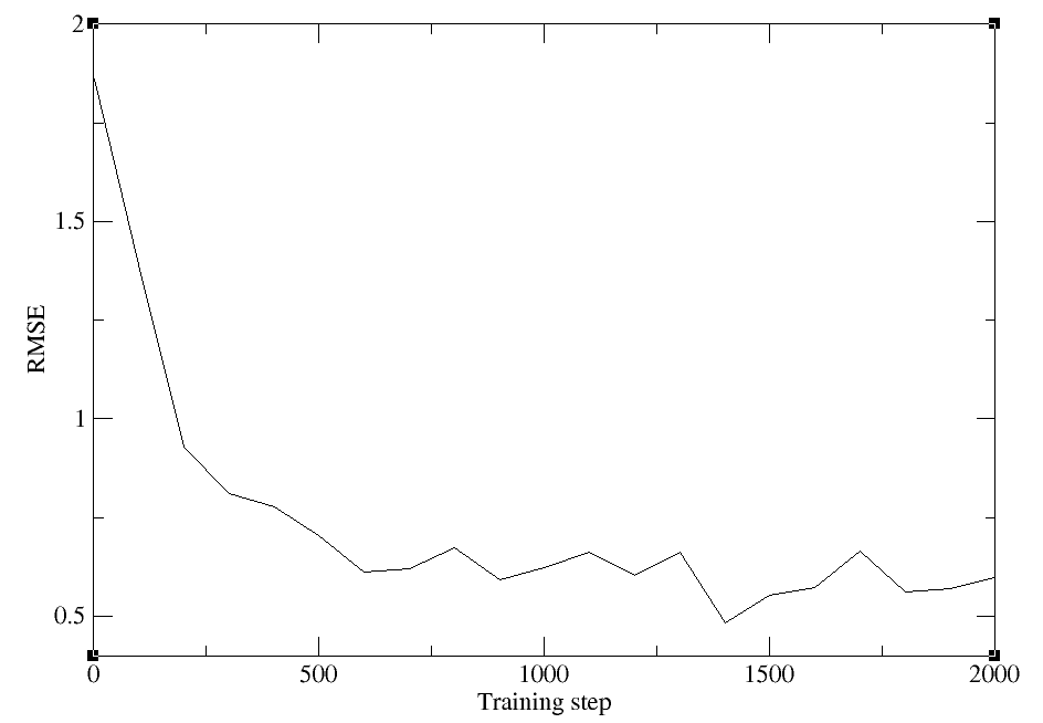
The training should take less than 10 minutes. In the process the train.log and lcurve.out files should populate. When it is available, take a look at lcurve.out, which tracks the loss:
 head c094a1e30c827c6dec19d3fb8fb4f84e4a82a30a/000/lcurve.out
 # step       rmse_trn    rmse_e_trn    rmse_f_trn   lr
# If there is no available reference data, rmse_*_{val,trn} will print nan
      1      1.86e+00      1.35e-04      1.86e-01    1.0e-03
    100      1.39e+00      2.88e-03      1.39e-01    1.0e-03
    200      9.28e-01      5.43e-04      9.26e-02    7.9e-04
    300      8.12e-01      2.91e-04      8.11e-02    6.3e-04
    400      7.78e-01      1.46e-04      7.78e-02    5.0e-04
    500      7.04e-01      1.85e-04      7.04e-02    4.0e-04
    600      6.11e-01      9.11e-05      6.10e-02    3.2e-04
    700      6.19e-01      1.01e-05      6.19e-02    2.5e-04
The columns correspond to the training step (here we will run 2000 steps), the overall trainin error, the error in the energy term, the error in the force term, and the learning rate, which scales over the training.
When the training has completed, intermediate files will be removed, and the outputs will be copied to iter.000001/00.train. The model deviation step will eventually fail because we are only training a single model, so these errors can be ignored once the training has completed. Navigate to the trainining directory and verify that your training has concluded sucessfully:
cd iter.000001/00.train
ls
000  data.hdf5  data.iters  graph.000.pth

cd 000
ls
checkpoint  frozen_model.pth  input.json  lcurve.out  model.ckpt.pt  old  train.log

grep -r "average training time:" train.log
[2026-02-04 10:38:17,404] DEEPMD INFO    average training time: 0.1061 s/batch

tail lcurve.out
1100      6.61e-01      4.08e-04      6.56e-02    1.0e-04
1200      6.02e-01      1.18e-04      6.01e-02    7.9e-05
1300      6.61e-01      2.55e-04      6.59e-02    6.3e-05
1400      4.82e-01      1.12e-04      4.81e-02    5.0e-05
1500      5.53e-01      2.48e-04      5.50e-02    4.0e-05
1600      5.72e-01      7.40e-05      5.72e-02    3.2e-05
1700      6.64e-01      2.98e-04      6.61e-02    2.5e-05
1800      5.62e-01      1.56e-04      5.61e-02    2.0e-05
1900      5.70e-01      1.95e-05      5.70e-02    1.6e-05
2000      5.97e-01      1.26e-04      5.97e-02    1.3e-05
We see that our model has been stored in graph.000.pth, the average timing has been reported in train.log, and see have reached 2000 steps in lcurve.out.
Even with a short training, we should see that the loss has decreased. Plot the total loss with xmgrace:
{{xmgraceload}}
xmgrace -block lcurve.out -bxy 1:2
The outputs can be downloaded here:
Attention
11.3.5. Model validation
Now we will use dp test to validate the training set as well as a test set. For the sake of computational expense, we will use data from the second umbrella as the test set. DP test will output the predicted force and energy corrections compared to the actual values stored in the hdf5 file. Download and navigate to the dptest directory where you have been provided a script called test_models.sh:
pwd
HandsOn11-Train_inputs/Train/SRP

cd dptest
Here are the contents of test_models.slurm:
#!/bin/bash
#SBATCH --partition={{GPUpartition}}
#SBATCH --job-name="model_eval"
#SBATCH --output=dptest.out
#SBATCH --error=dptest.err
#SBATCH --nodes=1
#SBATCH --ntasks-per-node=1
#SBATCH --cpus-per-task=1
#SBATCH --gpus-per-node=1
#SBATCH --time=0-00:30:00
#SBATCH --mem=8G


{{deepmdload}}

# Training set
dp test -m ../iter.000001/00.train/graph.000.pth -s ../common/img001_DFTB3.hdf5 -d parity_TrainingSet  2>&1 | tee dptest_TrainingSet.out
# Test set
dp test -m ../iter.000001/00.train/graph.000.pth -s ../common/img002_DFTB3.hdf5 -d parity_TestSet  2>&1 | tee dptest_TestSet.out
Run dp test, This should take less than 5 minutes.
sbatch test_models.slurm
The errors for every sample will be written to standard output. When the job is complete, take a look at the outputs:
head parity_TrainingSet.f.out
# ../common/img001_DFTB3.hdf5#/C15H16HW100N13O2OW51mC82mCl0mH97mN38mNa6mO46mP6: data_fx data_fy data_fz pred_fx pred_fy pred_fz
-2.466142177581787109e-05 -1.112073659896850586e-04 1.159161329269409180e-04 3.054524768231203780e-06 3.561235189408762380e-06 -2.306260057594045065e-06
-1.084312796592712402e-03 -1.249641180038452148e-03 1.153349876403808594e-03 3.313105116831138730e-05 -1.401095214532688260e-04 4.553010512609034777e-05
6.721727550029754639e-04 -2.709150314331054688e-03 -1.417696475982666016e-04 -7.833027048036456108e-04 6.616767495870590210e-04 -9.980606846511363983e-04
-4.771947860717773438e-04 2.542465925216674805e-03 -1.394093036651611328e-03 1.910269027575850487e-03 -2.701113931834697723e-03 2.913397504016757011e-03
-5.411714315414428711e-03 1.503229141235351562e-03 3.334641456604003906e-03 4.188372986391186714e-05 -3.068845020607113838e-03 9.139326866716146469e-04
3.090775012969970703e-02 5.400029942393302917e-03 -1.879560947418212891e-02 1.384735107421875000e-02 -3.181982785463333130e-02 1.924343779683113098e-02
-1.811271905899047852e-02 8.609175682067871094e-03 4.196822643280029297e-03 -2.041579410433769226e-02 -7.022037636488676071e-03 -9.910331107676029205e-03
-3.618022799491882324e-02 -3.521728515625000000e-02 -2.010071277618408203e-02 4.838545341044664383e-03 -2.629999816417694092e-02 3.696813806891441345e-02
4.276752471923828125e-03 -9.536743164062500000e-06 -3.337264060974121094e-03 1.505715423263609409e-03 -1.232840149896219373e-04 -3.571693378034979105e-05


head parity_TrainingSet.e.out
# ../common/img001_DFTB3.hdf5#/C15H16HW100N13O2OW51mC82mCl0mH97mN38mNa6mO46mP6: data_e pred_e
-3.903901417748034146e+04 -3.903902587962966936e+04
# ../common/img001_DFTB3.hdf5#/C15H16HW100N13O2OW52mC82mCl0mH94mN37mNa6mO46mP7: data_e pred_e
-3.903900805880523694e+04 -3.903890305559826811e+04
# ../common/img001_DFTB3.hdf5#/C15H16HW102N13O2OW47mC85mCl0mH94mN36mNa5mO46mP7: data_e pred_e
-3.903941908546729246e+04 -3.903946912129033444e+04
# ../common/img001_DFTB3.hdf5#/C15H16HW102N13O2OW55mC88mCl0mH96mN37mNa6mO48mP7: data_e pred_e
-3.903935605574178044e+04 -3.903914135217208241e+04
# ../common/img001_DFTB3.hdf5#/C15H16HW104N13O2OW53mC85mCl0mH90mN36mNa6mO50mP7: data_e pred_e
-3.903910261423454358e+04 -3.903933464041115803e+04
The forces are provided with x, y, z components, units are eV for energies and eV/angstrom for forces. The virial (v) is also provided, but we will focus on forces and energies because these were the components of our loss function. You have been provided the script plot_parity.py to plot the errors in the energies and magnitude of forces.
python plot_parity.py -f parity_TrainingSet.f.out -e parity_TrainingSet.e.out -l 'Train' -f parity_TestSet.f.out -e parity_TestSet.e.out -l 'Test' -s MTR1
Forces:
R2: 0.945
RMSE: 1.636
MAE: 0.703
Energies:
R2: 0.404
RMSE: 2.837
MAE: 2.316
----------
Forces:
R2: 0.945
RMSE: 1.639
MAE: 0.7
Energies:
R2: 0.079
RMSE: 3.491
MAE: 2.877
----------
The plot should look something like this:
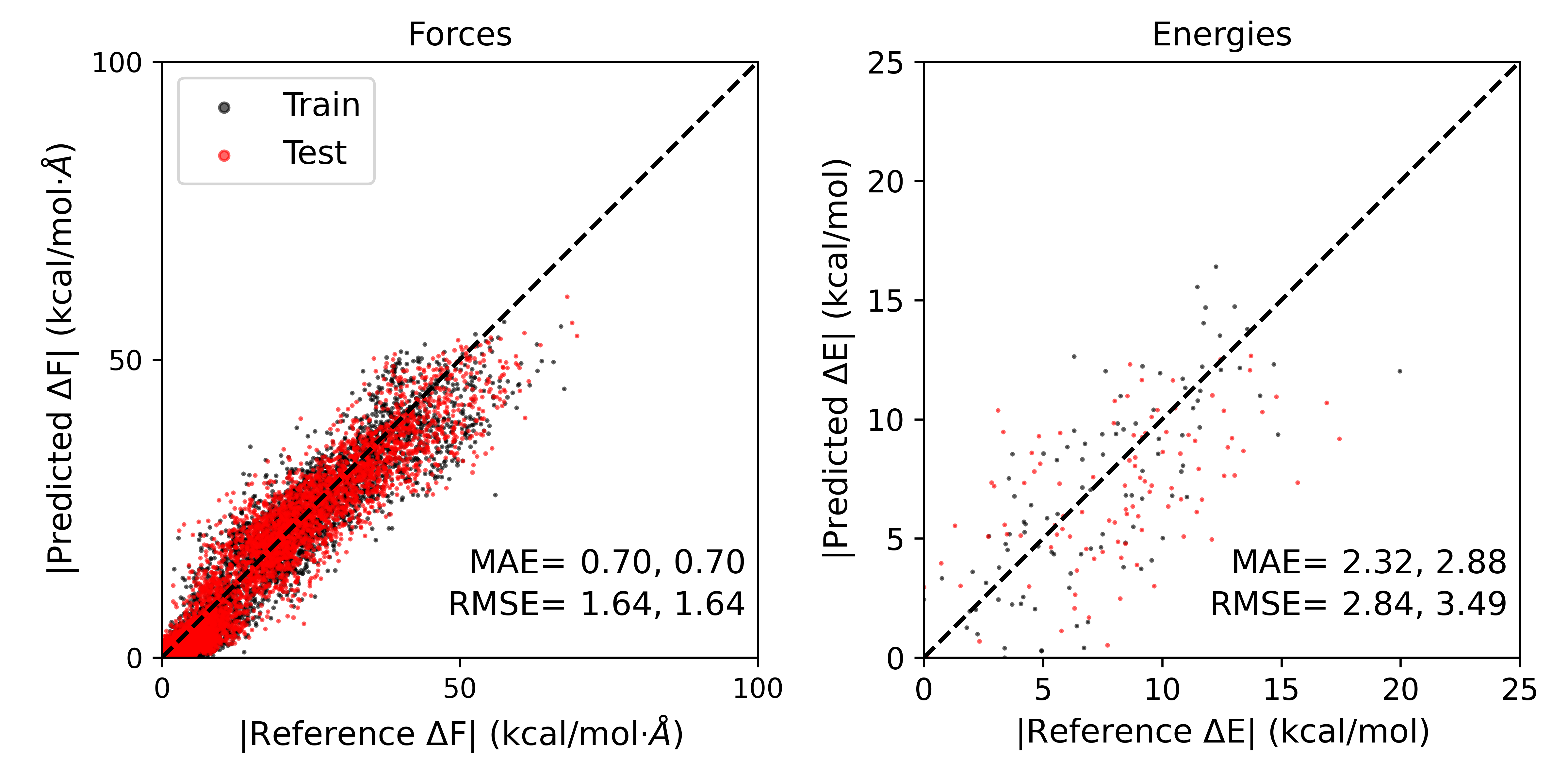
The errors obtained might be slightly different from independent training runs. The errors reported are given as Train,Test. As we can see, the errors for the test set are slightly higher than the training set, but both are quite low.
The outputs can be downloaded here:
Attention
11.3.6. Apply transfer learning
Now we implement transfer learning by initiating our model from a pre-trained foundational model.
Navigate to the Refine directory:
cd HandsOn11-Train_inputs/Train/Refine
ls
Foundation_model  common  computerprofiles  dptest  simplify_MACE.json
The pre-trained model file is stored in Foundation_model/00.train/000, and “training_init_model”: true directs the program to read in this model rather than initiating the model with random weights and biases. simplfy_MACE.json has been modifed to reflect this:
{
  "default_training_param": {
    "model": {
      "type": "mace",
      "type_map": ["C","H","N","O","P","Mg","Ca","Na","Zn","S","HW","OW","mC","mCl","mH","mMg","mN","mNa","mO","mP","mS"],
      "r_max": 6.0,
      "sel": 128,
      "num_radial_basis": 8,
      "num_cutoff_basis": 5,
      "max_ell": 3,
      "interaction": "RealAgnosticResidualInteractionBlock",
      "num_interactions": 2,
      "hidden_irreps": "128x0e + 128x1o",
      "pair_repulsion": false,
      "distance_transform": "None",
      "correlation": 3,
      "gate": "silu",
      "MLP_irreps": "16x0e",
      "radial_type": "bessel",
      "radial_MLP": [
        64,
        64,
        64
      ]
    },
    "learning_rate": {
      "type": "exp",
      "start_lr": 0.001,
      "decay_steps": 2000,
      "stop_lr": 1e-05
    },
    "loss": {
      "type": "ener",
      "start_pref_e": 1,
      "limit_pref_e": 100,
      "start_pref_f": 100,
      "limit_pref_f": 100,
      "start_pref_v": 0,
      "limit_pref_v": 0
    },
    "training": {
      "numb_steps": 2000,
      "disp_file": "lcurve.out",
      "disp_freq": 100,
      "save_freq": 1000,
      "disp_training": true,
      "time_training": true,
      "profiling": false,
      "profiling_file": "timeline.json"
    }
  },
  "type_map": ["C","H","N","O","P","Mg","Ca","Na","Zn","S","HW","OW","mC","mCl","mH","mMg","mN","mNa","mO","mP","mS"],
  "pick_data": "common/img001_DFTB3.hdf5",
  "training_init_model": true,
  "training_iter0_model_path": ["Foundation_model/00.train/000"],
  "sys_configs": [],
  "sys_batch_size": ["auto"],
  "init_pick_number": 20000,
  "iter_pick_number": 10000,
  "numb_models": 1,
  "training_reuse_iter": 2,
  "training_reuse_start_lr": 0.001,
  "training_reuse_old_ratio": "auto",
  "training_reuse_numb_steps": 100000,
  "training_reuse_start_pref_e": 1,
  "training_reuse_start_pref_f": 100,
  "dp_compress": false,
  "model_devi_f_trust_lo": 0.08,
  "model_devi_f_trust_hi": 2.0,
  "labeled": true,
  "init_data_sys": [],
  "init_data_prefix": "",
  "fp_task_min": 0,
  "mlp_engine": "dp",
  "one_h5": true,
  "train_backend": "pytorch"
}
Train the model using the same procedure in the previous section:
dpgen simplify simplify_MACE.json computerprofiles/machine_simplify.json 2>&1 | tee simplify.out
INFO:dpgen:start simplifying
INFO:dpgen:=============================iter.000000==============================
INFO:dpgen:-------------------------iter.000000 task 00--------------------------
INFO:dpgen:-------------------------iter.000000 task 01--------------------------
INFO:dpgen:first iter, skip step 1-5
INFO:dpgen:-------------------------iter.000000 task 02--------------------------
INFO:dpgen:first iter, skip step 1-5
INFO:dpgen:-------------------------iter.000000 task 03--------------------------
When it is complete, run dp test and plot the results:
cd dptest
sbatch test_models.slurm

...

python plot_parity.py -f parity_TrainingSet.f.out -e parity_TrainingSet.e.out -l 'Train' -f parity_TestSet.f.out -e parity_TestSet.e.out -l 'Test' -s MTR1
Forces:
R2: 0.998
RMSE: 0.303
MAE: 0.193
Energies:
R2: 0.919
RMSE: 1.046
MAE: 0.852
----------
Forces:
R2: 0.998
RMSE: 0.344
MAE: 0.209
Energies:
R2: 0.852
RMSE: 1.398
MAE: 1.116
----------
The results should look something like this:
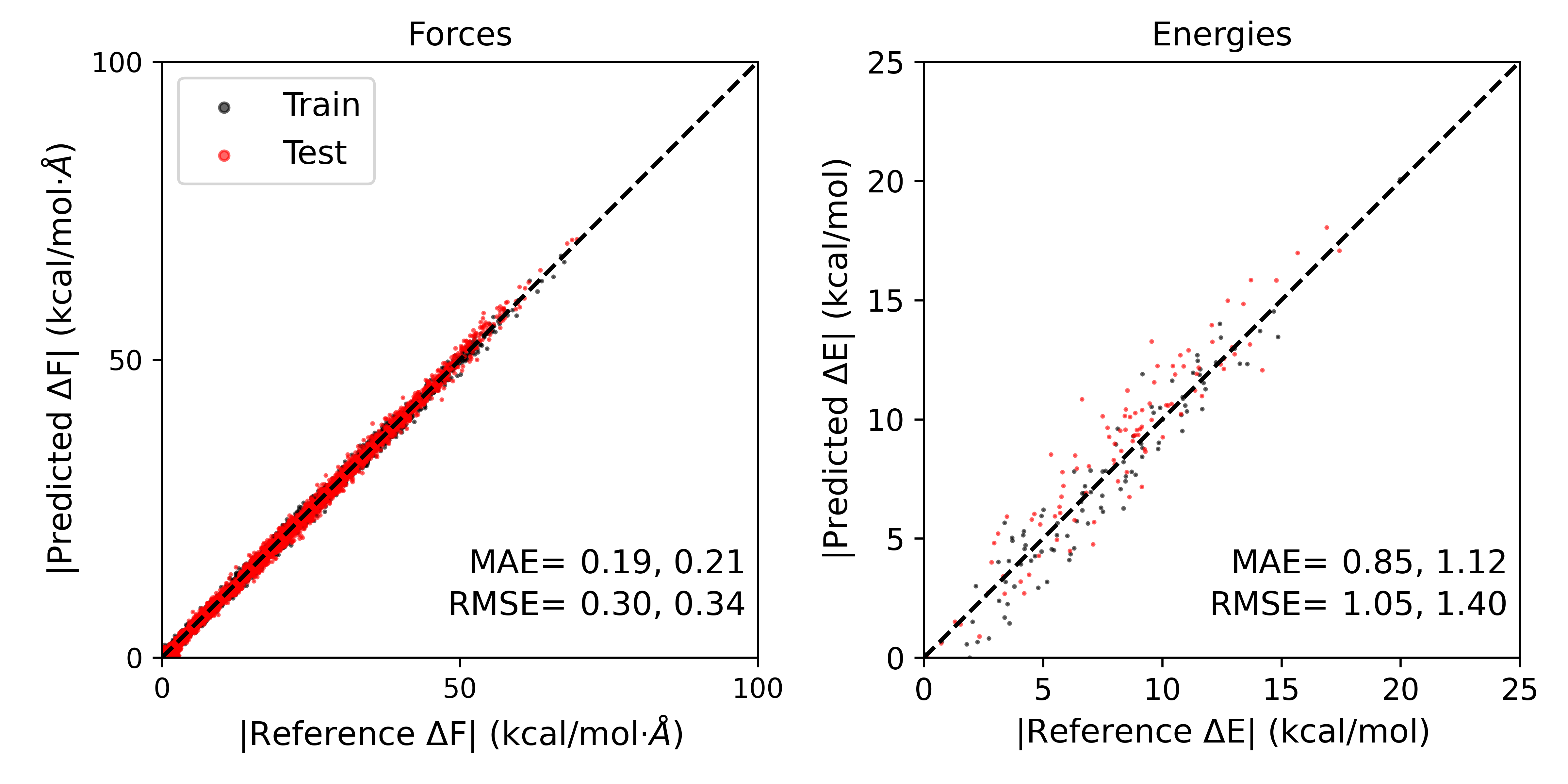
The errors in forces and energies for the training and test sets, even with very few training steps, have been significantly reduced by implementing transfer learning.
Attention
11.3.7. Model deviation for data-efficient active learning
There are two potential active learning approaches one could take using the DPGEN program in DeePMD-kit. These are “dpgen simplify” and “dpgen run”. Dpgen simplify is a pool-based active learning approach where an existing pool of data has already been labeld at the high level with single point calculations, and data is iteratively drawn from the pool for training. This is an active learning procedure because at each iteration, we compute a metric referred to as model deviation. Model deviation is a measure of uncertainty in the force predictions by a committee of stochastically trained models. The remaining pool is reduced before drawning new samples by removing samples for which the models already agree well, indicating high certainty in the estimate. In this way, training is focused on areas of greater uncertainty, and removing redundancy from the data set reduces the amount of training necessary.
The model deviation process is automated in dpgen simplify, but in this section we will do it by hand to demonstrate how the uncertainty estimate promotes efficient training. In pool-based avtive learning, model deviation would be computed for the entire pool to prune the number of samples availble for training in the next iteration. For the sake of this activity, we will take the img002 data as the pool. For the specific reaction potential and the refined potential, you have been provied the 3 additional replicas of the model that have been trained with the same procedure, but initiated from independent, stochastic initial states. Download the model-devi directory for the SRP model and navigate to it:
cd HandsOn11-Train_inputs/Train/SRP/model-devi
ls
graph.000.pth  graph.001.pth  graph.002.pth  graph.003.pth  img002_DFTB3.hdf5  model-devi.slurm   plot_modeldevi.py
You have been provided model-devi.slurm to compute the deviation in forces predicted by the four models. Here are the contents of model-devi.slurm:
#!/bin/bash
#SBATCH --partition={{GPUpartition}}
#SBATCH --job-name="model_devi"
#SBATCH --output=dpmodeldevi.out
#SBATCH --error=dpmodeldevi.err
#SBATCH --nodes=1
#SBATCH --ntasks-per-node=1
#SBATCH --cpus-per-task=1
#SBATCH --gpus-per-node=1
#SBATCH --time=0-00:30:00
#SBATCH --mem=8G


{{deepmdload}}


time dp model-devi -m graph* -s ../common/img002_DFTB3.hdf5 -o model-devi_SRP.out
Submit the job, which should complete in under 5 minutes:
sbatch model-devi.slurm
In the meantime, compute the model deviation for the refined model:
cd ../../Refine/model-devi
sbatch model-devi.slurm
Take a look at the output in model-devi_Refine.out:
head model-devi_Refine.out
# img002_DFTB3.hdf5#/C15H16HW100N13O2OW47mC87mCl0mH98mN37mNa6mO55mP7
# step      max_devi_v         min_devi_v         avg_devi_v         max_devi_f         min_devi_f         avg_devi_f         devi_e
          0       3.340329e-04       1.328199e-04       2.359955e-04       4.042720e-02       9.702322e-09       4.536546e-03       2.945244e-05
# img002_DFTB3.hdf5#/C15H16HW100N13O2OW49mC82mCl0mH97mN35mNa6mO54mP7
# step      max_devi_v         min_devi_v         avg_devi_v         max_devi_f         min_devi_f         avg_devi_f         devi_e
          0       3.974781e-04       8.601793e-05       2.444289e-04       3.997536e-02       8.229504e-11       4.046020e-03       3.907553e-05
# img002_DFTB3.hdf5#/C15H16HW100N13O2OW49mC84mCl0mH94mN35mNa6mO51mP8
# step      max_devi_v         min_devi_v         avg_devi_v         max_devi_f         min_devi_f         avg_devi_f         devi_e
          0       5.629255e-04       7.516243e-05       2.851215e-04       6.032073e-02       5.259309e-10       5.036927e-03       5.452317e-05
# img002_DFTB3.hdf5#/C15H16HW101N13O2OW50mC82mCl0mH95mN36mNa6mO51mP7
Remember that in the training input file we set model_devi_f_trust_lo to 0.08 ev/angstrom and model_devi_f_trust_hi to 2.0 eV/angstrom. This means any samples in the pool with maximum deviation in forces below model_devi_f_trust_lo or above model_devi_f_trust_hi will be removed from the pool.
We will use this metric to calculate how many samples would remain in the pool after your short training. In the HandsOn11/Train/SRP/model-devi directory you have been provided a script called plot_modeldevi.py. This will extract the max_devi_f column from the output. Run the script to compare the results of the SRP and the refined potential:
python plot_modeldevi.py -f model-devi_SRP.out -l 'SRP' -f ../../Refine/model-devi/model-devi_Refine.out -l 'Refine'
The result should look something like this:
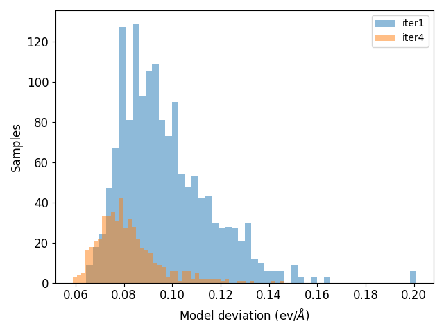
The black vertial line indicates model_devi_f_trust_lo. We can see that with the SRP, the models agree poorly, thus there is high uncertainty in the estimate. These samples would remain in the pool for further training in a pool-based active learning procedure. For the refined model, all samples fall below model_devi_f_trust_lo, indicating high certainty for this model and accurate results. These samples would be removed from the pool, thus saving time and resources training on redundant data. Taken together, the transfer learning process helps us achieve better accuracy quicker, and the model deviation based active learning approach improves data efficicency.
Attention
11.3.8. Addtional activity: on-the-fly active learning
Between hands on session 4 and the preceeding sections of this activity, you now have hands on experience running every component of an on-the-fly active learning procedure. This differs from pool-based active learning where the high level data has been precomputed. In this approach we will generate data “on-the-fly” by simulating the system with the version of the model trained in the last iteration. Therefore, the structures will be generated at a level of theory that increasingly mimics the target. Using the concept of model deviation, samples will be selected for further labeling with single point calculations. The prgram in DeePMD-Kit for this procedure is dpgen run.
This is a more computationally intensive approach than pool-based active learning, therefore you will learn to set up the calculations, and the resulting model will be provided for you to analyze.
The files for this section are in the AL directory:
ls HandsOn11-Train_inputs/Train/AL
Foundation_model  common  computerprofiles  generator.json  iter.000000  record.dpgen  restarts
You now have been provided an updated version of iter.000000 which points to the Foundation_model graph files. We must use 4 models for active learning, as model deviation cannot be computed with only one model.
You also have a new input file called generator.json. This has new inputs related to the model deviation and fp steps:
  ...

  "training_init_model": true,
  "training_iter0_model_path": ["Foundation_model/00.train/000", "Foundation_model/00.train/001", "Foundation_model/00.train/002", "Foundation_model/00.train/003"],
  "sys_configs": [
    [
      "/PATH2/AL/restarts/img001.rst7"
    ]
  ],
  "sys_batch_size": [
    "auto"
  ],
  "numb_models": 4,
  "training_reuse_iter": 2,
  "training_reuse_start_lr": 0.001,
  "training_reuse_old_ratio": "auto",
  "training_reuse_numb_steps": 2000,
  "training_reuse_start_pref_e": 0.02,
  "training_reuse_start_pref_f": 1000,
  "dp_compress": false,
  "model_devi_f_trust_lo": 0.08,
  "model_devi_f_trust_hi": 2.0,
  "labeled": true,
  "init_data_sys": [
    "img001_DFTB3.hdf5"
  ],
  "init_data_prefix": "common",
  "fp_task_min": 10,
  "mlp_engine": "dp",
  "one_h5": true,
  "train_backend": "pytorch",
  "mass_map": [12,1,14,16,31,24,40,23,65,32,1,16,12,35,1,24,14,23,16,31,32],
  "qm_region": [
    ":69|@272-282,290-291,1975-1988"
  ],
  "qm_charge": [
    1
  ],
  "parm7": [
    "/PATH2/AL/common/MTR.parm7"
  ],
  "mdin": [
    "/PATH2/AL/common/ml.mdin"
  ],
  "disang": [
    "/PATH2/AL/common/MTR.disang"
  ],
  "r": [
    [
      [
        -0.85970438,
        -1.7447896
      ]
    ]
  ],
  "nsteps": [
    2000
  ],
  "fp_task_max": 500,
  "fp_params": {
    "low_level_mdin": "/PATH2/AL/common/lowlevel.mdin",
    "high_level_mdin": "/PATH2/AL/common/highlevel.mdin"
  },
  "low_level": "DFTB3",
  "high_level": "PBE0",
  "cutoff": 6.0,
  "sys_format": "amber/rst7",
  "init_multi_systems": true,
  "model_devi_clean_traj": false,
  "model_devi_engine": "amber",
  "model_devi_skip": 0,
  "shuffle_poscar": false,
  "fp_style": "amber/diff",
  "detailed_report_make_fp": true,
  "use_clusters": true,
  "model_devi_jobs": [
    {
      "_comment": 0,
      "sys_idx": [
        0
      ],
      "trj_freq": 20
    }
  ]
}
Be sure to replace the PATH2 placeholder with your full working path.
The default training parameters are the same. Now we must provide inputs for how QM/MM simulations will be run, including restart file, reaction coordinate values, output frequency, the qm region, the qm charge, and the level of theory. In this example, the input is set up to run 2 additional active learning iterations based on the length of “model_devi_jobs”. We must also provide template file where the values will be inserted, which are located in common:
ls common
MTR.disang  MTR.parm7  highlevel.mdin  img001_DFTB3.hdf5 img002_DFTB3.hdf5 lowlevel.mdin  ml.mdin
lowlevel.mdin and highlevel.mdin will look familar from the first section of this activity, and ml.mdin will look familar from Hands on session 4. The mdin files contain place holders for inputs given in the json file, as this procedure could be used for multiple systems.
You have also been provided a new machine file called computerfile/machine_generator.json, which must allocate resources for QM/MM simulations and single point calculations:
{
  "train": [
    {
      "command": "dp",
      "machine": {
        "batch_type": "SlurmJobArray",
        "context_type": "LocalContext",
        "local_root": "./",
        "remote_root": "./"
      },
      "resources": {
        "number_node": 1,
        "cpu_per_node": 1,
        "gpu_per_node": 1,
        "custom_flags": [
          "#SBATCH --mem=32G",
          "#SBATCH --time=24:00:00",
          "#SBATCH --requeue",
        ],
        "module_list": [
          "{{deepmdload}}"
        ],
        "envs": {
          "OMP_NUM_THREADS": 1,
          "TF_INTER_OP_PARALLELISM_THREADS": 1,
          "TF_INTRA_OP_PARALLELISM_THREADS": 1
        },
        "group_size": 1,
        "queue_name": "{{GPUpartition}}"
      }
    }
  ],
  "model_devi": [
    {
      "command": "mpirun -n 1 sander.MPI",
      "group_size": 1,
      "machine": {
        "batch_type": "SlurmJobArray",
        "clean_asynchronously": true,
        "context_type": "LocalContext",
        "local_root": "./",
        "remote_root": "./"
      },
      "resources": {
        "number_node": 1,
        "gpu_per_node": 1,
        "cpu_per_node": 1,
        "custom_flags": [
          "#SBATCH --ntasks-per-node=1",
          "#SBATCH --mem=24G",
          "#SBATCH --time=24:00:00",
          "#SBATCH --requeue"
        ],
        "envs": {
          "OMP_NUM_THREADS": 1,
          "TF_INTER_OP_PARALLELISM_THREADS": 1,
          "TF_INTRA_OP_PARALLELISM_THREADS": 1
        },
        "group_size": 128,
        "queue_name": "{{GPUpartition}}",
        "module_list": [
          "{{amberload}}"
        ]
      }
    }
  ],
  "prepare": [
    {
      "command": "dp",
      "machine": {
        "batch_type": "Slurm",
        "context_type": "LocalContext",
        "local_root": "./",
        "remote_root": "./",
        "clean_asynchronously": true
      },
      "resources": {
        "number_node": 1,
        "cpu_per_node": 1,
        "gpu_per_node": 0,
        "custom_flags": [
          "#SBATCH -c 1",
          "#SBATCH --mem=8G",
          "#SBATCH --time=6:00:00",
          "#SBATCH --requeue"
        ],
        "module_list": [
          "{{deepmdload}}"
        ],
        "envs": {
          "OMP_NUM_THREADS": 1,
          "TF_INTER_OP_PARALLELISM_THREADS": 1,
          "TF_INTRA_OP_PARALLELISM_THREADS": 1
        },
        "group_size": 1,
        "queue_name": "{{CPUpartition}}"
      }
    }
  ],
  "fp": [
    {
      "command": "mpirun -n 4 sander.MPI",
      "machine": {
        "batch_type": "Slurm",
        "clean_asynchronously": true,
        "context_type": "LocalContext",
        "local_root": "./",
        "remote_root": "./"
      },
      "resources": {
        "cpu_per_node": 4,
        "gpu_per_node": 1,
        "custom_flags": [
          "#SBATCH --ntasks-per-node=4",
          "#SBATCH --mem=48G",
          "#SBATCH --time=48:00:00",
          "#SBATCH --requeue"
        ],
        "group_size": 50,
        "number_node": 1,
        "queue_name": "{{GPUpartition}}",
        "module_list": [
          "{{amberload}}",
          "{{deepmdload}}"
        ]
      }
    }
  ]
}
This approach would require multiple GPUs, so it will be run for you, but you have previously seen each component.
The job would be launched as follows:
dpgen run -d generator.json computerprofiles/machine_generator.json 2>&1 | tee generator.out
INFO:dpgen:start running
INFO:dpgen:continue from iter 000 task 02
INFO:dpgen:=============================iter.000000==============================
INFO:dpgen:-------------------------iter.000000 task 03--------------------------
INFO:dpgen:-------------------------iter.000000 task 04--------------------------

...
Download the outputs here to populate the results (some large file such as trajectories and mdfrc files have been removed for size):
Attention
The first step that will be performed is model deviation. This will be computed by running a simulation with the model trained in the first iteration training step. The template mdin file called ml.mdin in the common directory is used to write init0.rst7 such that model deviation is calculated and output in the mdout file. You can see what this looks like:
cd iter.000000/01.model_devi
tail init0.mdin
&dprc
  idprc=1
  mask=":69|@272-282,290-291,1975-1988"
  rcut = 6.0
  interfile(1)="../graph.000.pth"
  interfile(2)="../graph.001.pth"
  interfile(3)="../graph.002.pth"
  interfile(4)="../graph.003.pth"
/

cd task.000.000000
ls
TEMPLATE.disang  TEMPLATE.dumpave  init.rst7  job.json  rc.mdout  rc.nc  rc.rst7

grep -r "Active learning" rc.mdout | head -n1
Active learning frame written with max. frc. std.:     1.39740 kcal/mol/A
By specifying 4 models in the mdin file, 1 model is used to propogate dynamics, and the deviation in forces for each frame between the models is written to the mdout. This process generates candidates for labeling the single point calculations.
Next, navigate to the 02.fp directory and inspect the output:
cd ../../02.fp
ls
candidate.shuffled.000.out  low_level0.mdin                 rest_failed.shuffled.000.out  task.000.000003  task.000.000007  task.000.000011
data.000                    qm_region                       task.000.000000               task.000.000004  task.000.000008
high_level0.mdin            qmmm0.parm7                     task.000.000001               task.000.000005  task.000.000009
init0.rst7                  rest_accurate.shuffled.000.out  task.000.000002               task.000.000006  task.000.000010


cat candidate.shuffled.000.out
iter.000000/01.model_devi/task.000.000000 73
iter.000000/01.model_devi/task.000.000000 58
iter.000000/01.model_devi/task.000.000000 39
iter.000000/01.model_devi/task.000.000000 78
iter.000000/01.model_devi/task.000.000000 85
iter.000000/01.model_devi/task.000.000000 60
iter.000000/01.model_devi/task.000.000000 92
iter.000000/01.model_devi/task.000.000000 44
iter.000000/01.model_devi/task.000.000000 46
iter.000000/01.model_devi/task.000.000000 27
iter.000000/01.model_devi/task.000.000000 35
iter.000000/01.model_devi/task.000.000000 89


cd task.000.000000
ls
dataset  high_level.mdfrc  high_level.mdout  init.rst7  job.json  low_level.mdfrc  low_level.mdout  output  rc.nc
41 frames from the simulation were deemed candiates based on model deviation and will be subject to low and high level single point calculations. These are performed in the task diretories. You have already performed sinlge point calculation in the beginning of this exercise, except here it has been automated by DeePMD-Kit.
This candidate selection process is reflected in dpgen.log:
2026-02-12 11:54:17,687 - INFO : start running
2026-02-12 11:54:17,698 - INFO : continue from iter 000 task 02
2026-02-12 11:54:17,698 - INFO : =============================iter.000000==============================
2026-02-12 11:54:17,698 - INFO : -------------------------iter.000000 task 03--------------------------
2026-02-12 11:54:17,757 - INFO : -------------------------iter.000000 task 04--------------------------
2026-02-12 12:36:22,008 - INFO : -------------------------iter.000000 task 05--------------------------
2026-02-12 12:36:22,009 - INFO : -------------------------iter.000000 task 06--------------------------
2026-02-12 12:36:22,040 - INFO : system 000 candidate :     12 in    100  12.00 %
2026-02-12 12:36:22,041 - INFO : system 000 failed    :      0 in    100   0.00 %
2026-02-12 12:36:22,041 - INFO : system 000 accurate  :     88 in    100  88.00 %
2026-02-12 12:36:22,042 - INFO : system 000 accurate_ratio:   0.8800    thresholds: 1.0000 and 1.0000   eff. task min and max   -1  500   number of fp tasks:     12
2026-02-12 12:36:22,999 - INFO : -------------------------iter.000000 task 07--------------------------
2026-02-12 14:08:57,928 - INFO : -------------------------iter.000000 task 08--------------------------
2026-02-12 14:08:59,176 - INFO : failed tasks:      0 in     12    0.00 %
2026-02-12 14:08:59,177 - INFO : =============================iter.000001==============================
2026-02-12 14:08:59,177 - INFO : -------------------------iter.000001 task 00--------------------------
2026-02-12 14:08:59,177 - INFO : Use automatic training_reuse_old_ratio to make new-to-old ratio close to 10 times of the default value.
2026-02-12 14:09:01,141 - INFO : Combining 112 training systems to iter.000001/00.train/data.hdf5...
2026-02-12 14:09:01,815 - INFO : -------------------------iter.000001 task 01--------------------------
2026-02-12 14:15:07,842 - INFO : -------------------------iter.000001 task 02--------------------------
2026-02-12 14:15:07,847 - INFO : -------------------------iter.000001 task 03--------------------------
2026-02-12 14:15:07,848 - INFO : finished
After adding new single point calculations to the data set with the on the fly active learning approach, let’s see how the model performs. Navigate to the dptest directory and run dptest:
cd ../../dptest
sbatch test_models.slurm
When the job is done, plot the result:
python plot_parity.py -f parity_TrainingSet.f.out -e parity_TrainingSet.e.out -l 'Train' -f parity_TestSet.f.out -e parity_TestSet.e.out -l 'Test' -s MTR1
Forces:
R2: 0.998
RMSE: 0.309
MAE: 0.196
Energies:
R2: 0.9
RMSE: 1.16
MAE: 0.96
----------
Forces:
R2: 0.998
RMSE: 0.348
MAE: 0.212
Energies:
R2: 0.847
RMSE: 1.423
MAE: 1.124
----------
The result should look like this:

The errors obtained remain very small, even with a small number of training steps and a small dataset. In this case however, we have obtained comparable errors to pool based active learning by performing only 12 single point calculations, saving computational expense compared to the pool based approach because we have benefited from transfer learning. While this case was relatively simple, on-the-fly active learning can be especially effective if novel geometries or structures are observed at the ab initio level compared to the semi-empirical level.
The output can be downloaded here:
Attention