4. Hands-On Session 4: Calculating Free Energy Surfaces Using QM/MM-Δ Machine Learning Potentials
4.1. Learning Objectives
Select appropriate QM region and reaction coordinate definitions for your mechanistic question
Prepare the parameters and topology file for QM/MM simulations
Identify differences in the mdin file for running QM/MM versus MM, and how to apply a ΔMLP
Benchmark the difference in speeds for running semi-empirical, ΔMLP, and DFT level QM/MM
Perform umbrella sampling of a 1-dimensional reaction with AMBER
Use the NDFES program to produce a free energy profile with error bars
Interpret the free energy profile in the context of reaction mechanism
Verify that the ΔMLP free energy profile matches the DFT level
Demonstrate the importance of phase space overlap in umbrella window spacing for generating robust free energy profiles
4.2. Relevant literature
4.3. Activities
4.3.1. Workflow
        flowchart LR

%% ===== build the QM system =====
mm_files["mm.parm7<br/>mm.rst7"]
mm2qmmm{{"<b>[§4.3.2]</b><br/>Build the QM system<br/>mm2qmmm.py"}}
qmmm_files["<b>[from §4.3.2]</b><br/>QM/MM topology and coordinates<br/>qmmm.parm7<br/>qmmm.rst7"]
mm_files --> mm2qmmm
mm2qmmm --> qmmm_files

%% ===== preparing the inputs / window generation =====
templates["img.disang<br/>short.mdin<br/>reactant.disang<br/>product.disang"]
prepguess{{"<b>[§4.3.3]</b><br/>Generate umbrella windows<br/>ndfes-path-prepguess"}}
windows["<b>[from §4.3.3]</b><br/>Per-window restraints and inputs<br/>img01..32.disang<br/>img01..32.mdin"]
templates --> prepguess
qmmm_files --> prepguess
prepguess --> windows

%% ===== equilibrating the umbrella windows =====
sander_eq{{"<b>[§4.3.4]</b><br/>Equilibrate the windows<br/>sander.MPI"}}
init_rst["<b>[from §4.3.4]</b><br/>Equilibrated window restarts<br/>init01..32.rst7"]
windows --> sander_eq
qmmm_files --> sander_eq
sander_eq --> init_rst

%% ===== running umbrella sampling (DFTB3) =====
sander_dftb{{"<b>[§4.3.5]</b><br/>Run DFTB3 umbrella sampling<br/>sander.MPI"}}
init_rst --> sander_dftb
qmmm_files --> sander_dftb
windows --> sander_dftb

%% ===== applying a delta-machine learning potential =====
graph_file["graph.000.pth<br/>long_mlp.mdin"]
sander_mlp{{"<b>[§4.3.6]</b><br/>Run delta-MLP umbrella sampling<br/>sander.MPI"}}
init_rst --> sander_mlp
qmmm_files --> sander_mlp
windows --> sander_mlp
graph_file --> sander_mlp

%% ===== ab initio DFT potential with QUICK =====
sander_quick{{"<b>[§4.3.7]</b><br/>Run PBE0 timing simulation<br/>sander.MPI with QUICK"}}
init_rst --> sander_quick
qmmm_files --> sander_quick

%% ===== generating a free energy profile with NDFES =====
dumpave["<b>[from §4.3.5 and §4.3.6]</b><br/>Reaction coordinate samples<br/>img01..32.dumpave"]
prepdata{{"<b>[§4.3.8]</b><br/>Prepare data and metafile<br/>ndfes-PrepareAmberData"}}
metafile["<b>[from §4.3.8]</b><br/>Window metadata<br/>metafile"]
mbar{{"<b>[§4.3.8]</b><br/>Solve MBAR equations<br/>ndfes.OMP"}}
metafile_chk["<b>[from §4.3.8]</b><br/>Per-bin free energies<br/>metafile.chk"]
ndfes_path{{"<b>[§4.3.8]</b><br/>Compute PMF along path<br/>ndfes-path.OMP"}}
path_out["<b>[from §4.3.8]</b><br/>Free energy profile<br/>path.rbf.0.dat"]
sander_dftb --> dumpave
sander_mlp --> dumpave
dumpave --> prepdata
prepdata --> metafile
metafile --> mbar
mbar --> metafile_chk
metafile_chk --> ndfes_path
metafile --> ndfes_path
ndfes_path --> path_out

%% ===== combining sampling to generate a full PMF =====
full_pmf{{"<b>[§4.3.9]</b><br/>Combine windows for full PMF<br/>ndfes-path.OMP"}}
full_pmf_out["<b>[from §4.3.9]</b><br/>Full reaction PMF<br/>path_all.rbf.0.dat"]
metafile_chk --> full_pmf
full_pmf --> full_pmf_out

classDef file fill:#fff7e6,stroke:#d98c00,stroke-width:1.5px,color:#111;
classDef program fill:#e8f1ff,stroke:#1f77b4,stroke-width:1.8px,color:#111;
classDef result fill:#eaf7ea,stroke:#2ca02c,stroke-width:1.5px,color:#111;
class mm_files,templates,graph_file file;
class mm2qmmm,prepguess,sander_eq,sander_dftb,sander_mlp,sander_quick,prepdata,mbar,ndfes_path,full_pmf program;
class qmmm_files,windows,init_rst,dumpave,metafile,metafile_chk,path_out,full_pmf_out result;
4.3.2. Build the QM system - 1D methyl transfer in MTR1
Download the necessary inputs for this activity:
Attention
Copy the directory to your working directory
cp -r /PATH2Files/HandsOn4-FESurface_inputs.tar.gz ./
tar -xzvf HandsOn4-FESurface_inputs.tar.gz
cd HandsOn4-FESurface_inputs
Load the amber module:
{{amberload}}
You will also periodically need to use xmgrace to plot your results. Load the xmgrace module:
{{xmgraceload}}
The motivation for using umbrella sampling is that, without restraints, a system undergoing dynamics will very rarely cross a reaction barrier. Even if it does, it will be very sparsely sampled and take much longer than we can afford to sample. Therefore, we apply a series of harmonic biasing potentials, also referred to as an umbrella potential, to force the system over a free energy barrier in the space of the selected reaction coordinate. In this way, we can thoroughly sample the breaking and formation of bonds, or other processes like a conformational change. In order to construct a potential of mean force, we must track the value of the reaction coordinate throughout our simulations so that we can later remove the impact of the bias and compute what the distribution of sampling would look like had we not applied the restraint. This activity will show you how to perform and analyze QM/MM simulations of a methyl transfer reaction in the MTR1 ribozyme using 1 reaction coordinate.
The active site is shown in Figure 1, and includes the methyl donor ligand (O6 methylated guanine), the nucleophillic target A63, and C10 protonated at the N3 position.
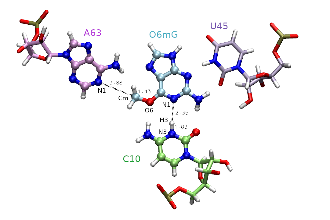
First, we must decide which atoms will be treated quantum mechanically (aka the QM region). The rest of the atoms will be treated with the molecular mechanical force field. In this case, we are simulating methyl transfer from O6 methylated guanine (O6mG) to the N1 of A63, so we want to include both of these residues in the QM region. The positively charged C10 residue is directly hydrogen bonding to the leaving group, so we will include it as well. In the next activity this residue will also be involved in the reaction, so we will proactively include it now. For A63 and C10, we will only include the nucleobases since the backbones are not directly involved in the reaction. Additionally, U45 is important for holding the ligand in the active site, but since it is not directly involved in the reaction it will remain in the MM region. Based on this selection, the total charge of the QM region is +1 because C10 is in a non-standard protonation state.
Based on this QM region selection, we need to make some modifications to the parameter and topology files. These include: * remove connection atom charges at the QM/MM interface * redistribute MM charges so that the QM region within each residues is integer * remove Ewald atoms from TIP4P-Ew MM waters to be included in the QM region * remove any dummy atoms if present * add Lennard Jones parameters to QM atoms that lack then in MM (ie H’s)
Navigate to the mm2qmmm directory.
cd mm2qmmm
ls
mm.parm7  mm.rst7  mm2qmmm.py
The equilibrated mm.parm7 and mm.rst7 files have been provied for you along with the script mm2qmmm.py. This script will convert the mm parameter and topology files for use with QM/MM. Display the scripts options:
python mm2qmmm.py -h
usage: mm2qmmm.py [-h] -p PARM -c CRD -q QMCHARGE -m QMMASK -o OPARM -r ORST

Converts MM parameter/restart files to versions appropriate for QM/MM.
It removes connection atom charges, and redistributes MM charges so
that the QM region within each residue is an integer. It removes
M-sites from QM waters and removes dummy particles used in pKa
calculations. It adds LJ parameters to QM atoms that lack LJ
parameters in the MM representation.

optional arguments:
  -h, --help            show this help message and exit
  -p PARM, --parm PARM  MM parameter file
  -c CRD, --crd CRD     MM restart file
  -q QMCHARGE, --qmcharge QMCHARGE
                        QM charge
  -m QMMASK, --qmmask QMMASK
                        QM mask based on the MM parameter file representation
  -o OPARM, --oparm OPARM
                        QMMM output parameter file
  -r ORST, --orst ORST  QMMM output restart file
  -R, --hmr             (optional) if present, then repartition H-masses in the QM region and set the timestep to 2 fs
The QM mask corresponding to the bases of C9 and A62 and the O6mG cofactor is “:69|@272-282,290-291,1975-1988”, and the net QM charge is +1 due to the protonated C residue. We will also apply hydrogen mass repartitioning. This is required to safely run QM/MM with a 2 fs timestep. Run mm2qmmm.py:
python mm2qmmm.py -p mm.parm7 -c mm.rst7 -q 1 -m ":69|@272-282,290-291,1975-1988" -o qmmm.parm7 -r qmmm.rst7 --hmr
CHARGE GROUP: :9
CHARGE GROUP: :62
CHARGE GROUP: :69
BEFORE charge adjustments:
The net charge of     grp                   :9 is  -0.00000
The  QM charge within grp                   :9 is   0.90650
The  MM charge within grp                   :9 is  -0.90650
AFTER charge adjustments:
The net charge of     grp                   :9 is  -0.00000
The  QM charge within grp                   :9 is   1.00000
The  MM charge within grp                   :9 is  -1.00000

BEFORE charge adjustments:
The net charge of     grp                  :62 is  -1.00000
The  QM charge within grp                  :62 is  -0.12410
The  MM charge within grp                  :62 is  -0.87590
AFTER charge adjustments:
The net charge of     grp                  :62 is  -1.00000
The  QM charge within grp                  :62 is   0.00000
The  MM charge within grp                  :62 is  -1.00000

BEFORE charge adjustments:
The net charge of     grp                  :69 is  -0.00200
The  QM charge within grp                  :69 is  -0.00200
The  MM charge within grp                  :69 is   0.00000
AFTER charge adjustments:
The net charge of     grp                  :69 is   0.00000
The  QM charge within grp                  :69 is   0.00000
The  MM charge within grp                  :69 is   0.00000

The MM charges of the whole QM region is   1.00000
          The expected net QM charge is   1.00000

New LJ type for QM type N* using old parameters (rmin=  1.8240 eps=  0.1700): @272,278,290,1975,1978,1981,1984,1987
New LJ type for QM type C4 using old parameters (rmin=  1.9080 eps=  0.0860): @273,275,277,281,1976,1979,1980,1985,1988
New LJ type for QM type H4 using old parameters (rmin=  1.4090 eps=  0.0150): @274
New LJ type for QM type HA using old parameters (rmin=  1.4590 eps=  0.0150): @276
New LJ type for QM type  H using old parameters (rmin=  0.6000 eps=  0.0157): @279,280,291,1982,1983
New LJ type for QM type  O using old parameters (rmin=  1.6612 eps=  0.2100): @282
New LJ type for QM type H5 using old parameters (rmin=  1.3590 eps=  0.0150): @1977,1986
Adjusting nonbond pair:  7 ( N*) -  1 ( HO) (rmin=  1.8240 eps=  0.0771)
Adjusting nonbond pair:  8 ( C4) -  1 ( HO) (rmin=  1.9080 eps=  0.0549)
Adjusting nonbond pair:  9 ( H4) -  1 ( HO) (rmin=  1.4090 eps=  0.0229)
Adjusting nonbond pair: 10 ( HA) -  1 ( HO) (rmin=  1.4590 eps=  0.0229)
Adjusting nonbond pair: 11 (  H) -  1 ( HO) (rmin=  0.6000 eps=  0.0234)
Adjusting nonbond pair: 12 (  O) -  1 ( HO) (rmin=  1.6612 eps=  0.0857)
Adjusting nonbond pair: 14 ( H5) -  1 ( HO) (rmin=  1.3590 eps=  0.0229)
Adjusting nonbond pair: 15 ( os) -  1 ( HO) (rmin=  1.7713 eps=  0.0504)
Adjusting nonbond pair: 16 ( nc) -  1 ( HO) (rmin=  1.8993 eps=  0.0574)
Adjusting nonbond pair: 17 ( na) -  1 ( HO) (rmin=  1.7992 eps=  0.0845)
Adjusting nonbond pair: 18 ( nh) -  1 ( HO) (rmin=  1.7903 eps=  0.0867)
Adjusting nonbond pair: 19 ( ca) -  1 ( HO) (rmin=  1.8606 eps=  0.0588)
Adjusting nonbond pair: 20 ( c3) -  1 ( HO) (rmin=  1.9069 eps=  0.0614)
Adjusting nonbond pair: 21 ( h5) -  1 ( HO) (rmin=  1.3735 eps=  0.0237)
Adjusting nonbond pair: 22 ( h1) -  1 ( HO) (rmin=  1.3593 eps=  0.0270)
Adjusting nonbond pair: 23 ( hn) -  1 ( HO) (rmin=  0.6210 eps=  0.0187)
You should now have qmmm.parm7 and qmmm.rst7 files.
The outputs can be downloaded here:
Attention
4.3.3. Preparing the inputs
Navigate back to the base directory and copy the parm7 file to the template directory. Then copy the rst7 file to the directory called start.
cd ..
cp mm2qmmm/qmmm.parm7 template
cp mm2qmmm/qmmm.rst7 start/reactant.rst7
You have been provided a template mdin file (template/short.mdin). This mdin file is valid for QM/MM simulations in general, and is not specific to umbrella sampling. Let’s take a look at short.mdin:
short
&cntrl
! IO =======================================
      irest = 0       ! 0 = start, 1 = restart
        ntx = 1       ! 1 = start, 5 = restart
      ntxo = 1       ! read/write rst as formatted file
      iwrap = 1       ! wrap crds to unit cell
    ioutfm = 1       ! write mdcrd as netcdf
      imin = 0
      ntmin = 1
      ntpr = 20
      ntwr = 20
      ntwx = 0
      ntwf = 0
! DYNAMICS =================================
    nstlim = 250
        dt = 0.002   ! ps/step
        ntb = 1       ! 1=NVT periodic, 2=NPT periodic, 0=no box
! TEMPERATURE ==============================
      temp0 = 298     ! target temp
  gamma_ln = 5.0     ! Langevin collision freq
        ntt = 3       ! thermostat (3=Langevin)
! PRESSURE  ================================
        ntp = 0       ! 0=no scaling, 1=isotropic, 2=anisotropic
! SHAKE ====================================
        ntc = 2       ! 1=no shake, 2=HX constrained, 3=all constrained
noshakemask = ":69|@272-282,290-291,1975-1988"    ! do not shake these
        ntf = 1       ! 1=cpt all bond E, 2=ignore HX bond E, 3=ignore all bond E
! MISC =====================================
        cut = 10.0
      ifqnt = 1
        ig = -1
    nmropt = 1
/


&ewald
  dsum_tol = 1.e-6
/

&qmmm
    qm_theory   = 'DFTB3'
        qmmask  = ':69|@272-282,290-291,1975-1988'
      qmcharge  = 1
          spin  = 1
      qmshake  = 0
      qm_ewald  = 1
  qmmm_switch  = 1
      scfconv  = 1.e-10
    verbosity  = 0
  tight_p_conv  = 1
  diag_routine  = 0
  pseudo_diag  = 1
  dftb_maxiter  = 100
/


&wt type = 'DUMPFREQ', istep1 = 10, /
&wt type='END' /
DISANG=img.disang
DUMPAVE=img.dumpave
LISTOUT=POUT
LISTIN=POUT
The timestep (dt) is set to 0.002 ps, or 2 fs. We will only perform short simulations of 0.5 ps to start in order to generate the windows, therfore nstlim is set to 250.
We will be using the DFTB3 semi-empirical Hamiltonian, and the total charge of the QM region is +1 due to the protonation of cytosine. When determining the total charge of a nucleic acid QM region, be sure to consider any negatively charged phosphates that may be included. The QM region is defined by the mask ‘:69|@272-282,290-291,1975-1988’ which includes the entire ligand (:69), the nucleobase of C10 (@272-282,290-291) and the nucleobase of A63 (@1975-1988).
The noshakemask contains the same mask as the QM region, thus we will not shake QM atoms as these bonds involving hydrogen may fluctuate outside of equilibrium MM values when bonds are made/broken. SHAKE constraints are inherently dependent on the MM force field, thus MM constraints should not be combined with our QM description.
Since we want to apply nmr restraints, nmropt is set to 1, and we will output restraint values to the dumpave file every 10 steps. The green highlighted img.disang and img.dumpave are place holders that will be replaced to indicate the appropriate umbrella window number in order to apply restraints.
Let’s review how nmr restraints work in AMBER. When nmropt=1 is set in the mdin file, restraints will be read from the specified DISANG file. These are different than coordinate restraints set when using ntr=1, which effectively freezes the atoms in place. Using nmr restraints allows the atom position to fluctuate subject to a specified biasing potential relating it to another atom or atoms. The values of the restrained properties for a given step are output to the specified DUMPAVE file with a frequency of istep1.
Next we need to select the reaction coordinates. We choose the reaction coordinate to be the difference in distance between the atoms where the bond will break, and between the atoms where the bond will form. This ensures the reaction coordinate value to increase going from reactant to product making it more intuitive. In MTR1, describing methyl transfer between O6mG:O6 and A63:N1 will yield the reaction coordinate (RC): RC = |RO6mG:O6 - RCm| - | RA63:N1 - RCm |. We will evaluate the reaction going from the reactant with RC at -2.5 Å, to product with RC at 2.5 Å. You have been provided template/img.disang containing the restraint definitions.
Take a look at img.disang:
#methylation: |GN-C5|-|A62-C5|
&rst iat= 2200, 2189, 2200, 1984,
r1=-999, r2=RC1, r3=RC1, r4=999, rk2=100, rk3=100, rstwt=1.0,-1.0 /

#Max distances for H-bonds

## 1 ##
&rst iat= 1403, 2207,
r1=-999, r2=-999, r3=3.00, r4=999,rk2=0, rk3=100 /

## 2 ##
&rst iat= 1405, 2192,
r1=-999, r2=-999, r3=2.20, r4=999,rk2=0, rk3=100 /

## 3 ##
&rst iat= 1407, 2206,
r1=-999, r2=-999, r3=2.00, r4=999,rk2=0, rk3=100 /

## 4 ##
&rst iat= 2205, 282,
r1=-999, r2=-999, r3=2.20, r4=999,rk2=0, rk3=100 /

## 5 ##
&rst iat= 280, 2189,
r1=-999, r2=-999, r3=2.20, r4=999,rk2=0, rk3=100 /

## 6 ##
&rst iat= 2190, 1982,
r2=-999, r2=-999, r3=3.00, r4=999,rk2=0, rk3=100 /

## 7 ##
&rst iat= 291, 2193,
r1=-999, r2=-999, r3=2.20, r4=999,rk2=0, rk3=100 /
For now, we need to understand more about the restraints used in this example. The first restraint defines the reaction coordinate. The line “&rst iat= 2200, 2189, 2200, 1984,” indicates that we are restraining the difference in distance between the methyl carbon (2200) to ligand oxygen (2189) and the methyl carbon (2200) to the N1 of adenine (1984). These distances are shown in Figure 1. The presence of “rstwt=1.0,-1.0” indicates this should be a difference of distances. In theory, the two distances could be seperate reaction coordinates, but combining them reduces the dimensionality while still describing the same event. The values of r1, r2, r3, and r4 define the shape of the biasing potential. The r2 and r3 values define the flat region of the potential. If r2 is less than r3, then there is no penalty for being within those bounds. When applying an umbrella potential, we set r2=r3 to sample directly on the desired value. The img.disang file is a template, where RC1 will ultimately be replaced for each umbrella window. If more reaction coordinates were present, the placeholder RC2 and so on would be used. The r1 and r4 values define the bounds of the linear response region, ie the penalty will progressively increase as the restrained property approaches r1 and r4. By setting r1=-999 and r4=999 we have effectively created a parabola with infinite bounds. The values rk2 and rk3 are the weights of the restraints. These effectively define the steepness of the parabola, thus controlling the penalty for going outside the r2 to r3 region. For umbrella sampling we want to set this to a high number to force the sampling of high energy regions. The higher the free energy at an umbrella center position, the more the observed value (reported in the dumpave file) will attempt to move away from this center and fight against the biasing potential. It is the concept that helps us construct a PMF.
The rest of the restraints do not define reaction coordinates, and they will be held constant in all of the umbrella windows. These are distance restraints on the active site hydrogen bonds to the ligand to ensure it stays in the pocket. These are different from the harmonic potential used for the reaction coordinate because r2=-999 and rk2=0. This defines a half-harmonic biasing potential where any distance less than 3.0 feels no penalty. If the values were reversed (ie. r3=999 and rk2=100), then the two atoms would be pushed away from each other. Now that we have a comprehensive understand of the nmr restraints, we will focus on setting up an umbrella sampling simulation.
Now we will generate the equil directory based on the inputs provided. This will be where we sequentially generate the umbrella windows starting from the reactant structure. It is important to slowly increment the reaction coordinate starting from a neighboring structure because each time you change the restraint, you are effectively changing the force field and risk large spikes in energy that could cause unintended bonds to break. We will use the ndfes program to write the inputs for this step.
You have been provided a reactant and product.disang file where the reaction coordinate is set to -2.5 and 2.5 respectively. These will define the end points, and a total of 32 umbrella windows will be generated to linearly interpolate through them.
Navigate to the start directory and run the following command.
cd start
ndfes-path-prepguess.py --disang ../template/img.disang --mdin ../template/short.mdin --min reactant.disang --min product.disang --nsim 32 --odir ../equil --pad 2 --dry-run
The –min flags indicate the minima we want to use as control points (reactant and product). The option –disang indicates the template disang file with a placeholder, –mdin indicates the template mdin file with a placeholder, –nsim determines the number of umbrella windows, and –pad means the file names will be padded with a leading zero. The –dry-run flag will just print the output without creating the simulation directory called equil. The output should look like this:
 1    -2.500   ../equil/img01.disang
 2    -2.339   ../equil/img02.disang
 3    -2.177   ../equil/img03.disang
 4    -2.016   ../equil/img04.disang
 5    -1.855   ../equil/img05.disang
 6    -1.694   ../equil/img06.disang
 7    -1.532   ../equil/img07.disang
 8    -1.371   ../equil/img08.disang
 9    -1.210   ../equil/img09.disang
10    -1.048   ../equil/img10.disang
11    -0.887   ../equil/img11.disang
12    -0.726   ../equil/img12.disang
13    -0.565   ../equil/img13.disang
14    -0.403   ../equil/img14.disang
15    -0.242   ../equil/img15.disang
16    -0.081   ../equil/img16.disang
17     0.081   ../equil/img17.disang
18     0.242   ../equil/img18.disang
19     0.403   ../equil/img19.disang
20     0.565   ../equil/img20.disang
21     0.726   ../equil/img21.disang
22     0.887   ../equil/img22.disang
23     1.048   ../equil/img23.disang
24     1.210   ../equil/img24.disang
25     1.371   ../equil/img25.disang
26     1.532   ../equil/img26.disang
27     1.694   ../equil/img27.disang
28     1.855   ../equil/img28.disang
29     2.016   ../equil/img29.disang
30     2.177   ../equil/img30.disang
31     2.339   ../equil/img31.disang
32     2.500   ../equil/img32.disang
dmax     0.161
dmax is the spacing between umbrella windows. In general, if the spacing is too large (>0.2), consider adding more windows. For our purposes this is sufficiently small.
Run the command again without the –dry-run flag to create the equil directory:
ndfes-path-prepguess.py --disang ../template/img.disang --mdin ../template/short.mdin --min reactant.disang --min product.disang --nsim 32 --odir ../equil --pad 2
The outputs can be downloaded here:
Attention
4.3.4. Equilibrating the umbrella windows
List the contents of the equil directory:
cd ../equil
ls
eq01fwd.sh    img04.disang  img07.mdin    img11.disang  img14.mdin    img18.disang  img21.mdin    img25.disang  img28.mdin    img32.disang
img01.disang  img04.mdin    img08.disang  img11.mdin    img15.disang  img18.mdin    img22.disang  img25.mdin    img29.disang  img32.mdin
img01.mdin    img05.disang  img08.mdin    img12.disang  img15.mdin    img19.disang  img22.mdin    img26.disang  img29.mdin    init01.rst7
img02.disang  img05.mdin    img09.disang  img12.mdin    img16.disang  img19.mdin    img23.disang  img26.mdin    img30.disang
img02.mdin    img06.disang  img09.mdin    img13.disang  img16.mdin    img20.disang  img23.mdin    img27.disang  img30.mdin
img03.disang  img06.mdin    img10.disang  img13.mdin    img17.disang  img20.mdin    img24.disang  img27.mdin    img31.disang
img03.mdin    img07.disang  img10.mdin    img14.disang  img17.mdin    img21.disang  img24.mdin    img28.disang  img31.mdin
You will see that the eq01fwd.sh script was generated for you in the ouputs directory.
Take a look at eq01fwd.sh:
#!/bin/bash
set -e
set -u

#
# You can create a slurm script and run these
# commands in the following way:
#
# export LAUNCH="srun sander.MPI"
# export PARM="path/to/parm7"
# bash eq01fwd.sh
#

if [ "${LAUNCH}" == "" ]; then
    echo 'bash variable LAUNCH is undefined. Defaulting to: export LAUNCH="sander"'
    export LAUNCH="sander"
fi

if [ "${PARM}" == "" ]; then
    echo 'bash variable PARM is undefined. Please: export PARM="/path/to/parm7"'
    exit 1
else
   if [ ! -e "${PARM}" ]; then
       echo "File not found: ${PARM}"
       exit 1
   fi
fi

if [ ! -e "init01.rst7" ]; then
    echo "File not found: init01.rst7"
    exit 1
fi

${LAUNCH} -O -p ${PARM} -i img01.mdin -o img01.mdout -c init01.rst7 -r img01.rst7 -x img01.nc -inf img01.mdinfo
${LAUNCH} -O -p ${PARM} -i img02.mdin -o img02.mdout -c img01.rst7 -r img02.rst7 -x img02.nc -inf img02.mdinfo
${LAUNCH} -O -p ${PARM} -i img03.mdin -o img03.mdout -c img02.rst7 -r img03.rst7 -x img03.nc -inf img03.mdinfo
${LAUNCH} -O -p ${PARM} -i img04.mdin -o img04.mdout -c img03.rst7 -r img04.rst7 -x img04.nc -inf img04.mdinfo
${LAUNCH} -O -p ${PARM} -i img05.mdin -o img05.mdout -c img04.rst7 -r img05.rst7 -x img05.nc -inf img05.mdinfo
${LAUNCH} -O -p ${PARM} -i img06.mdin -o img06.mdout -c img05.rst7 -r img06.rst7 -x img06.nc -inf img06.mdinfo
${LAUNCH} -O -p ${PARM} -i img07.mdin -o img07.mdout -c img06.rst7 -r img07.rst7 -x img07.nc -inf img07.mdinfo
${LAUNCH} -O -p ${PARM} -i img08.mdin -o img08.mdout -c img07.rst7 -r img08.rst7 -x img08.nc -inf img08.mdinfo
${LAUNCH} -O -p ${PARM} -i img09.mdin -o img09.mdout -c img08.rst7 -r img09.rst7 -x img09.nc -inf img09.mdinfo
${LAUNCH} -O -p ${PARM} -i img10.mdin -o img10.mdout -c img09.rst7 -r img10.rst7 -x img10.nc -inf img10.mdinfo
${LAUNCH} -O -p ${PARM} -i img11.mdin -o img11.mdout -c img10.rst7 -r img11.rst7 -x img11.nc -inf img11.mdinfo
${LAUNCH} -O -p ${PARM} -i img12.mdin -o img12.mdout -c img11.rst7 -r img12.rst7 -x img12.nc -inf img12.mdinfo
${LAUNCH} -O -p ${PARM} -i img13.mdin -o img13.mdout -c img12.rst7 -r img13.rst7 -x img13.nc -inf img13.mdinfo
${LAUNCH} -O -p ${PARM} -i img14.mdin -o img14.mdout -c img13.rst7 -r img14.rst7 -x img14.nc -inf img14.mdinfo
${LAUNCH} -O -p ${PARM} -i img15.mdin -o img15.mdout -c img14.rst7 -r img15.rst7 -x img15.nc -inf img15.mdinfo
${LAUNCH} -O -p ${PARM} -i img16.mdin -o img16.mdout -c img15.rst7 -r img16.rst7 -x img16.nc -inf img16.mdinfo
${LAUNCH} -O -p ${PARM} -i img17.mdin -o img17.mdout -c img16.rst7 -r img17.rst7 -x img17.nc -inf img17.mdinfo
${LAUNCH} -O -p ${PARM} -i img18.mdin -o img18.mdout -c img17.rst7 -r img18.rst7 -x img18.nc -inf img18.mdinfo
${LAUNCH} -O -p ${PARM} -i img19.mdin -o img19.mdout -c img18.rst7 -r img19.rst7 -x img19.nc -inf img19.mdinfo
${LAUNCH} -O -p ${PARM} -i img20.mdin -o img20.mdout -c img19.rst7 -r img20.rst7 -x img20.nc -inf img20.mdinfo
${LAUNCH} -O -p ${PARM} -i img21.mdin -o img21.mdout -c img20.rst7 -r img21.rst7 -x img21.nc -inf img21.mdinfo
${LAUNCH} -O -p ${PARM} -i img22.mdin -o img22.mdout -c img21.rst7 -r img22.rst7 -x img22.nc -inf img22.mdinfo
${LAUNCH} -O -p ${PARM} -i img23.mdin -o img23.mdout -c img22.rst7 -r img23.rst7 -x img23.nc -inf img23.mdinfo
${LAUNCH} -O -p ${PARM} -i img24.mdin -o img24.mdout -c img23.rst7 -r img24.rst7 -x img24.nc -inf img24.mdinfo
${LAUNCH} -O -p ${PARM} -i img25.mdin -o img25.mdout -c img24.rst7 -r img25.rst7 -x img25.nc -inf img25.mdinfo
${LAUNCH} -O -p ${PARM} -i img26.mdin -o img26.mdout -c img25.rst7 -r img26.rst7 -x img26.nc -inf img26.mdinfo
${LAUNCH} -O -p ${PARM} -i img27.mdin -o img27.mdout -c img26.rst7 -r img27.rst7 -x img27.nc -inf img27.mdinfo
${LAUNCH} -O -p ${PARM} -i img28.mdin -o img28.mdout -c img27.rst7 -r img28.rst7 -x img28.nc -inf img28.mdinfo
${LAUNCH} -O -p ${PARM} -i img29.mdin -o img29.mdout -c img28.rst7 -r img29.rst7 -x img29.nc -inf img29.mdinfo
${LAUNCH} -O -p ${PARM} -i img30.mdin -o img30.mdout -c img29.rst7 -r img30.rst7 -x img30.nc -inf img30.mdinfo
${LAUNCH} -O -p ${PARM} -i img31.mdin -o img31.mdout -c img30.rst7 -r img31.rst7 -x img31.nc -inf img31.mdinfo
${LAUNCH} -O -p ${PARM} -i img32.mdin -o img32.mdout -c img31.rst7 -r img32.rst7 -x img32.nc -inf img32.mdinfo
This script would start from img01 and iteratively generate the umbrella windows using the output of the previous window as the starting structure. It is important to increment the starting structure slowly to avoid errors. The serial nature of this process makes it too slow to compute during the course of this workshop, so these simulations have been conducted for you.
4.3.5. Running umbrella sampling
After generating the windows, it is a best practice to exclude the first ~2 ps of production sampling from analysis to allow for proper equilibration time. The equilibration region can be checked using ndfes-CheckEquil.py. However, under the time constraints of the exercise, you will not be able to perform long enough sampling to gather equilibrium statistics, so you will only perform enough sampling to generate a PMF.
Now we will perform umbrella sampling using DFTB3 on all of the umbrella windows in parallel. For the sake of of this exercise, the windows have been divided into 8 groups of 4 in directories called t1 through t8. Normally, one would run all of the windows together, but this will allow each participant to perform 3 ps of sampling in ~8 minutes. This activity will focus on t1 as an example, but any of the 8 could be selected.
Navigate to the DFTB3 directory and list the contents of the t1 directory:
cd DFTB3
ls t1
analyze_1-4.sh  img01.mdin    img02.mdin    img03.mdin    img04.mdin   init02.rst7  init04.rst7    template.groupfile
img01.disang    img02.disang  img03.disang  img04.disang  init01.rst7  init03.rst7  run_1-4.slurm
The init{01..04} restart files are copies of the final img{01..04} restart files generated in the equil directory. In the mdin files, nstlim has been increased to 1500 so that with a 2 fs timestep we will perform 3 ps of sampling. It is typically desirable to run longer simulations when more time is available; however, this will be enough sampling to generate and analyze a PMF as a demonstration.
You have also been provided a slurm script called run_1-4.slurm.
Take a look at run_1-4.slurm:
#!/bin/bash
#SBATCH --job-name="sim.1-4"
#SBATCH --output="%a.slurmout"
#SBATCH --error="%a.slurmerr"
#SBATCH --partition={{CPUpartition}}
#SBATCH --nodes=1
#SBATCH --ntasks-per-node=32
#SBATCH --mem=64GB
#SBATCH --cpus-per-task=1
#SBATCH --requeue
#SBATCH --export=ALL
#SBATCH -t 0-00:30:00
#SBATCH --account={{account}}

{{amberload}}

export LAUNCH="srun --mpi=pmi2 -K1 -N1 -n32 -c1 --exclusive sander.MPI"

set -e
set -u


$LAUNCH -ng 4 -groupfile template.groupfile
wait
sleep 1
Each window will be allotted 8 cores. Now that the jobs are being run in parallel, we will provide a groupfile as input to sander.MPI.
Take a look at the groupfile:
-O -p ../../template/qmmm.parm7 -c init01.rst7 -i img01.mdin -o img01.mdout -r img01.rst7 -x img01.nc -inf img01.mdinfo
-O -p ../../template/qmmm.parm7 -c init02.rst7 -i img02.mdin -o img02.mdout -r img02.rst7 -x img02.nc -inf img02.mdinfo
-O -p ../../template/qmmm.parm7 -c init03.rst7 -i img03.mdin -o img03.mdout -r img03.rst7 -x img03.nc -inf img03.mdinfo
-O -p ../../template/qmmm.parm7 -c init04.rst7 -i img04.mdin -o img04.mdout -r img04.rst7 -x img04.nc -inf img04.mdinfo
This is similar to executing multiple backgrounded (&) sander.MPI processes, but it also gives us the capability to run replica exchange if desired.
Navigate to your trial directory and submit the job:
cd t1
sbatch run_1-4.slurm
The outputs can be downloaded here:
Attention
4.3.6. Applying a Δ-machine learning potential
Now we will re-run the 4 window simulation applying a Δ machine learning potential (ΔMLP). This is a potential trained to correct a base model to a target level of theory. In this case the ΔMLP is trained to correct the DFTB3 potential to replicate the energies and forces obtained at the PBE0/6-31G* level. Specifically, the potential is a model fine-tuned for this reaction from a foundatinal MACE based ΔMLP for nucleic acid enzyme reactions. This process will be the suject of a later activity, and for now we will just appy the model.
In order to apply the ΔMLP, you will need a file containing the model parameters. In the template directory you have been provided a file called graph.000.pth. This is a python pickled object that contains the trained model parameters. The .pth extension means this is a model trained with PyTorch. You have also been provided a template mdin file called long_mlp.mdin. Take a look at this file:
MACE
&cntrl
! IO =======================================
      irest = 0       ! 0 = start, 1 = restart
      ntx = 1       ! 1 = start, 5 = restart
      ntxo = 1       ! read/write rst as formatted file
      iwrap = 1       ! wrap crds to unit cell
      ioutfm = 1       ! write mdcrd as netcdf
      imin = 0
      ntmin = 1
      ntpr = 20
      ntwr = 20
      ntwx = 0
      ntwf = 0
! DYNAMICS =================================
    nstlim = 1500
        dt = 0.002   ! ps/step
        ntb = 1       ! 1=NVT periodic, 2=NPT periodic, 0=no box
! TEMPERATURE ==============================
      temp0 = 298     ! target temp
  gamma_ln = 5.0     ! Langevin collision freq
        ntt = 3       ! thermostat (3=Langevin)
! PRESSURE  ================================
        ntp = 0       ! 0=no scaling, 1=isotropic, 2=anisotropic
! SHAKE ====================================
        ntc = 2       ! 1=no shake, 2=HX constrained, 3=all constrained
noshakemask = ":69|@272-282,290-291,1975-1988"    ! do not shake these
        ntf = 1       ! 1=cpt all bond E, 2=ignore HX bond E, 3=ignore all bond E
! MISC =====================================
        cut = 10.0
      ifqnt = 1
        ig = -1
    nmropt = 1
/


&ewald
  dsum_tol = 1.e-6
/

&ewald
  dsum_tol = 1.e-6
/

&qmmm
    qm_theory   = 'DFTB3'
        qmmask  = ':69|@272-282,290-291,1975-1988'
      qmcharge  = 1
          spin  = 1
      qmshake  = 0
      qm_ewald  = 1
  qmmm_switch  = 1
      scfconv  = 1.e-10
    verbosity  = 0
  tight_p_conv  = 1
  diag_routine  = 0
  pseudo_diag  = 1
  dftb_maxiter  = 100
/


&wt type = 'DUMPFREQ', istep1 = 5, /
&wt type='END' /
DISANG=img.disang
DUMPAVE=img.dumpave
LISTOUT=POUT
LISTIN=POUT

&dprc
  idprc=1
  mask=":69|@272-282,290-291,1975-1988"
  rcut = 6.0
  intrafile=""
  interfile(1)="../../template/graph.000.pth"
/
The input files are the same except for the additional dprc namelist. Because the base model is DFTB3, we must still specify DFTB3 as the QM theory. A ΔMLP should not be applied on top of a QM method it was not trained to correct. DPRC stands for Deep Potential Range Correction, meaning the correction is applied for QM-QM interactions and QM-MM interactions within an rcut radius of 6 angstroms, where the correction smoothly vanishes. The mask should match the qmmask, and interfile should point to the model file. The dprc correction is considered an “interfile” because it corrects QM-QM and QM-MM interactions, whereas an “intrafile” would be a model only correcting the internal QM potential. We leave this option blank. Multiple interfiles can be specified, in which case the deviation between the models is reported in the mdout. This is useful when training models with active learning, but for this application we will only use 1 model file.
Navigate to the dMLP directory and take a look at the run script for this set of 4 simulations:
cd dMLP/t1
cat run_1-4_MACE.slurm

#!/bin/bash
#SBATCH --job-name="sim.1-4.MACE"
#SBATCH --output="%a.slurmout"
#SBATCH --error="%a.slurmerr"
#SBATCH --partition={{GPUpartition}}
#SBATCH --nodes=1
#SBATCH --cpus-per-task=1
#SBATCH --ntasks-per-gpu=4
#SBATCH --mem=256G
#SBATCH --export=ALL
#SBATCH -t 0-00:30:00
#SBATCH --account={{account}}

{{amberload}}

export LAUNCH="srun --mpi=pmi2 -K1 -N1 -n4 -c1 --exclusive sander.MPI"

set -e
set -u


$LAUNCH -ng 4 -groupfile template.groupfile
wait
sleep 1
The ΔMLP inference is accelerate by GPUs, so we must request a GPU node. We will use 1 sander task per window because the underlying DFTB3 simulation is still performed by the CPU, and there are less CPUs present within the GPU node than a large CPU node.
Submit the job:
sbatch run_1-4_MACE.slurm
The outputs can be downloaded here:
Attention
4.3.7. Using an ab initio DFT potential with QUICK
Now we will use QUICK to perform a short simulation for a single window with the PBE0 Hamiltonian and 6-31G* basis set. Navigate to the PBE0 directory where you have been provided the required inputs:
cd PBE0
ls
img01.disang  img01.mdin  init01.rst7  run_PBE0.slurm
For PBE0 we will only run a single window for 2 steps to get timing info because ab initio DFT is more expensive than semi-empirical or ΔMLP level simulations. Let’s take a look at img01.mdin:
PBE0
&cntrl
! IO =======================================
      irest = 0       ! 0 = start, 1 = restart
        ntx = 1       ! 1 = start, 5 = restart
      ntxo = 1       ! read/write rst as formatted file
      iwrap = 1       ! wrap crds to unit cell
    ioutfm = 1       ! write mdcrd as netcdf
      imin = 0
      ntmin = 1
      ntpr = 1
      ntwr = 1
      ntwx = 1
      ntwf = 0
! DYNAMICS =================================
    nstlim = 1    ! number of time steps
        dt = 0.002   ! ps/step
        ntb = 1       ! 1=NVT periodic, 2=NPT periodic, 0=no box
! TEMPERATURE ==============================
      temp0 = 298     ! target temp
  gamma_ln = 5.0     ! Langevin collision freq
        ntt = 3       ! thermostat (3=Langevin)
! PRESSURE  ================================
        ntp = 0       ! 0=no scaling, 1=isotropic, 2=anisotropic
! SHAKE ====================================
        ntc = 2       ! 1=no shake, 2=HX constrained, 3=all constrained
noshakemask = ":69|@272-282,290-291,1975-1988"    ! do not shake these
        ntf = 1       ! 1=cpt all bond E, 2=ignore HX bond E, 3=ignore all bond E
! MISC =====================================
        cut = 10.0
      ifqnt = 1
        ig = -1
    nmropt = 1
/


&wt
type='DUMPFREQ', istep1=1
&end
&wt
  type='END',
&end
DISANG=img01.disang
DUMPAVE=img01.dumpave

&ewald
  dsum_tol = 1.e-6
/

&qmmm
    qm_theory   = 'quick'
        qmmask  = ':69|@272-282,290-291,1975-1988'
      qmcharge  = 1
          spin  = 1
      qmmm_int  = 1
      qm_ewald  = 1
      qmshake  = 0
        itrmax  = 50
      scfconv  = 1e-07
    verbosity  = 0
/

&quick
  method   = 'PBE0'
  basis    = '6-31G*'
/
Now we get the qm_theory to quick, which points to the &quick namelist where we specify the method and basis set. Now take a look at run_PBE0.slurm:
#!/bin/bash
#SBATCH --job-name="sim.PBE0"
#SBATCH --output="PBE0.slurmout"
#SBATCH --error="PBE0.slurmerr"
#SBATCH --partition=gpu-debug
#SBATCH --gpus=1
#SBATCH --nodes=1
#SBATCH --ntasks-per-gpu=16
#SBATCH --mem=24G
#SBATCH --cpus-per-task=1
#SBATCH --export=ALL
#SBATCH -t 0-00:30:00
#SBATCH --account=rut149

{{amberload}}

top=`pwd`
export LAUNCH="srun --mpi=pmi2 -n16 --exclusive"
export EXE="sander.MPI"

parm=../template/qmmm.parm7

time ${LAUNCH} ${EXE} -O -p ${parm} -c init01.rst7 -i img01.mdin -o img01.mdout -r img01.rst7 -x img01.nc -inf img01.mdinfo
QUICK is a GPU accelerated QM program, therefore we will request a GPU node, and 4 parallel tasks. We will also time the job to get a sense of the speed. Submit the job, which should finish within 20 minutes. During that time, feel free do the analysis in the next section while it runs.
sbatch run_PBE0.slurm
When the job is done, take a look at the timing:
tail -n3 PBE0.slurmerr
real  4m4.347s
user  0m0.011s
sys   0m0.035s
Compare this with the timings you get with DFTB3 and ΔMLP to get a sense of the speed-up enabled by the ΔMLP.
The outputs can be downloaded here:
Attention
4.3.8. Generating a free energy profile with NDFES
While the simulations are running, take a look at the analyze_1-4.sh script in the DFTB3 trial 1 directory:
#!/bin/bash

mkdir analysis
mkdir analysis/dumpaves

cd analysis

for i in $(seq 1 4); do

  base=$(printf "img%02i" ${i})
  ndfes-PrepareAmberData.py -d ../${base}.disang -i ../${base}.dumpave -o dumpaves/${base}.dumpave -r 1 >> metafile

done

ndfes.OMP --mbar -w 0.15 --nboot 0 -c metafile.chk metafile

ndfes-path.OMP --chk metafile.chk --ipath metafile --npathpts 4 --nsplpts 20 --opath path
This script will create an analysis directory and use the ndfes program to generate the potential of mean force for the segment of the reaction space spanned by your 4 umbrella windows. Each simulation generates a dumpave file that tracks the values of the restrained properties, including the reaction coordinate. For each dumpave file, the program ndfes-PrepareAmberData.py will extract just the data related to the reaction coordinate and output this to a new dumpave file in analysis/dumpaves. It will also generate a file called metafile that will indicate the index of the Hamiltonian (default is zero), the temperature (default is 298), the path to the dumpave file, the umbrella center, and the force constant.
Next, the program ndfes.OMP is used to solve the MBAR equations with a bin width equal to 0.15. Setting the –nboot flag equal to zero means that we will perform no bootstrap resamples. If you wish to put error bars on your data points, nboot can be set to a nonzero number like 50, but this analysis will take longer with more resamples. The output of the program is an xml file called metafile.chk. This contains the value of the free energy in each sampled bin.
Finally, we use the ndfes-path.OMP program to print the PMF information to a file called path. In this example, we are merely asking it to print the free energy along a path that is defined by the 4 control points in the metafile (ie. where we placed the umbrella windows). To create a smooth curve, we will use 20 spline points to represent our path. When using interpolation, the default setting is to use radial basis functions (rbf). Additional options will be discussed in upcoming exercises with more complex reaction paths.
When the simulations are complete, run the analysis script and take a look at the ouput.
bash analyze_1-4.sh
ls analysis
dumpaves  metafile  metafile.chk  path  path.rbf.0.dat  path.xml
Plot the path using xmgrace:
cd analysis
xmgrace -block path.rbf.0.dat -bxy 3:4
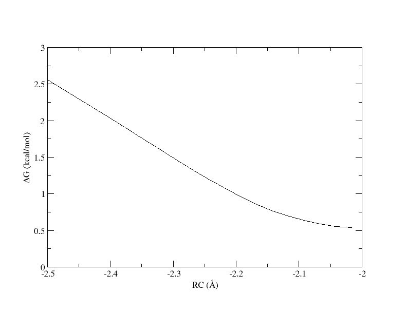
PMF as a function of reaction coordinate value from simulation of 4 umbrella windows.
The y-axis is the free energy in kcal/mol, and the x-axis is the reaction coordinate value. Without the context of the other umbrella windows, this does not give us much information. Now we will look at the PMF as a whole.
The outputs can be downloaded here:
Attention
4.3.9. Combining sampling to generate a full PMF
Now we will analyze the free energy profiles generated from the DFTB3 and ΔMLP simulations using the N-Dimensional Free Energy Surface (NDFES) program, which is available in AMBER tools. We will combine all of the umbrella sampling trials to construct a combined PMF. You have been provided the output of all of the trials that must be copied to the working directory.
Copy the remaining trial directories to your working directory.
Create a directory called combined_analysis.
List the contents of your working directory. It should be structured as follows:
cp -r INSERTPATH/QMMM_DFTB3_MTR1/1D/ouputs/t{2..8} ./
mkdir combined_analysis
ls
combined_analysis  t1  t2  t3  t4  t5  t6  t7  t8
The structure files have been removed from the output directories for the sake of file size, but these would have been generated by the simulations and are not required for analysis. We want to combine the metafiles from all of the trial directories.
Run the following command to generate metafile.all:
cd combined_analysis
ndfes-CombineMetafiles.py -o metafile.all ../t{1..8}/analysis/metafile
Run the following command to generate metafile.all.chk:
ndfes.OMP --mbar -w 0.15 --nboot 0 -c metafile.all.chk metafile.all
This will generate metafile.all.chk. Finally, we will generate the path file for the entire PMF.
Run the following command to generate the path file:
ndfes-path.OMP --chk metafile.all.chk --ipath metafile.all --npathpts 32 --nsplpts 400 --opath path_all
The ndfes commands are also given in combined_analysis.sh, but for the sake of understanding the role of each program they have been run one at a time.
Plot the PMF with xmgrace:
xmgrace -block path_all.rbf.0.dat -bxy 3:4
The outputs can be downloaded here:
Attention
Now we will repeat the analysis for the ΔMLP simulations to compare the our DFTB3 result.
cd ../dMLP
mkdir combined_analysis
cd combined_analysis
ndfes-CombineMetafiles.py -o metafile.all ../t{1..8}/analysis/metafile
ndfes.OMP --mbar -w 0.15 --nboot 0 -c metafile.all.chk metafile.all
ndfes-path.OMP --chk metafile.all.chk --ipath metafile.all --npathpts 32 --nsplpts 400 --opath path_all
The outputs can be downloaded here:
Attention
Finally, you have been provided the full outputs for 3 ps of sampling at the PBE0 level. Navigate to the PBE0 directory, and run analysis:
cd ../../PBE0/init
bash analyze.sh
The outputs can be downloaded here:
Attention
Now, plot the DFTB3, ΔMLP, and PBE0 level free energy profiles together using xmgrace:
cd ../../
xmgrace -block DFTB3/combined_analysis/path_all.rbf.0.dat -bxy 2:4 -block dMLP/combined_analysis/path_all.rbf.0.dat -bxy 2:4 -block PBE0/init/analysis/path.rbf.0.dat -bxy 2:4
The plot should look something like this:
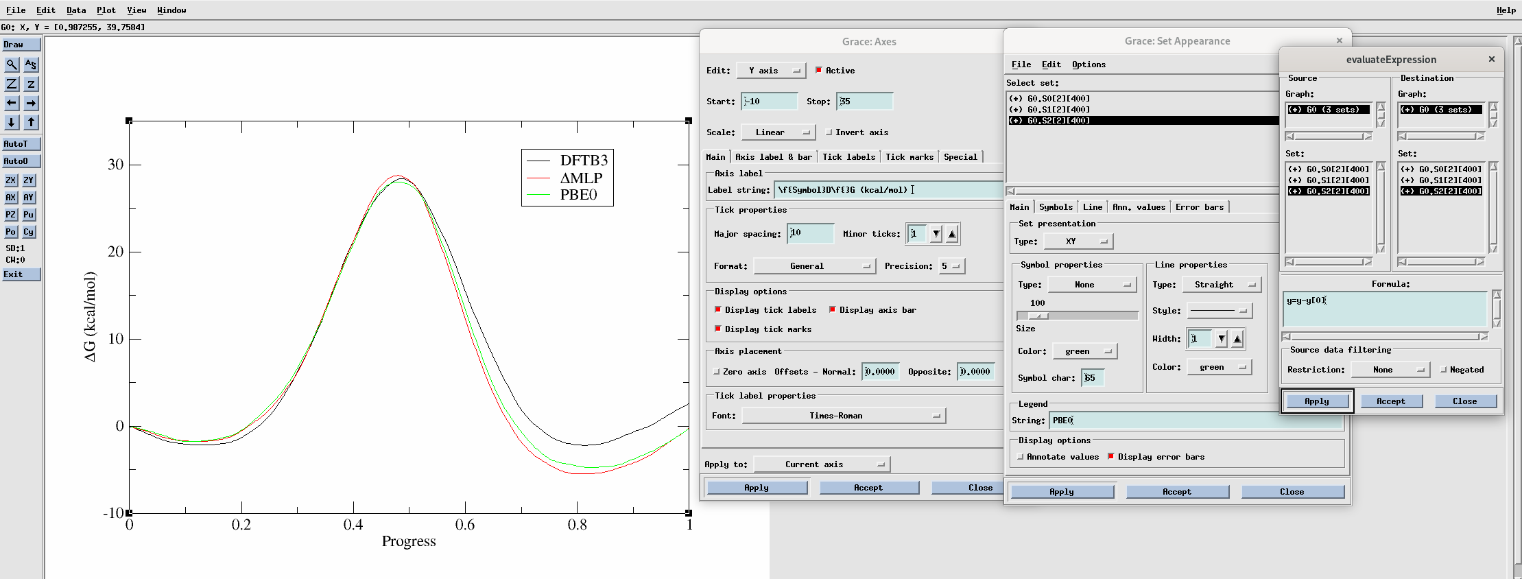
You can adjust the appearance of the plot using the settings shown in the above image. To align the plots such that the free energy of the initial point is zero, go to Data –> Transformations –> Evaluate expression and evaluate y = y - y[0] for each curve. To make the legend, go to Plot –> Set appearance. To modify the axes go to Plot –> Axis properties.
The ΔMLP result brings our profile much closer to the PBE0 result compared to DFTB3. All methods, however, yield a high free energy barrier of approximately 30 kcal/mol. This would yield an intrinsic rate estimate of approximately 3.7e-8 / min, which would render the activity almost undetectable. It looks likely that our mechanism is more complicated that simply transfering the methyl group. In 1 dimension it is very clear what the path is from reactants to products, and we can plot the free energy as a function of a single coordinate. However, if more reaction coordinates are involved, the path from reactant to product is less clear. In the following sections you will see how the use of more reaction coordinates can better model this reaction.
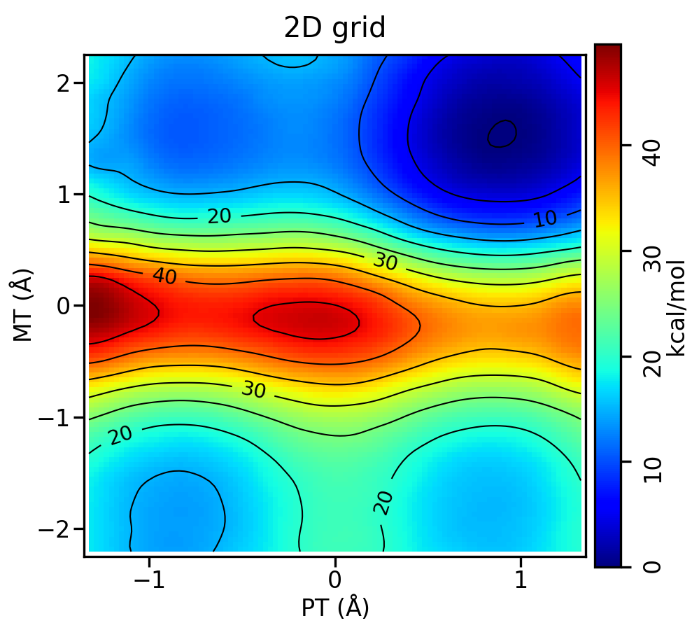
4.3.10. Additional exercise: computing a 2D free energy surface from a grid
The most straight-forward way to sample a multidimensional free energy surface is to construct a regular grid in the reaction coordinate space. Navigate to the Grid directory:
cd HandsOn4-FESurface_inputs/Grid
ls
prod analysis

cd prod
ls | head
img_-0.2p_-0.1m.disang
img_-0.2p_-0.1m.dumpave
img_-0.2p_-0.3m.disang
img_-0.2p_-0.3m.dumpave
img_-0.2p_-0.5m.disang
img_-0.2p_-0.5m.dumpave
img_-0.2p_-0.7m.disang
img_-0.2p_-0.7m.dumpave
img_-0.2p_-0.9m.disang

ls *disang | wc -l
286
You have been provided the output from a grid of ΔMLP simulations. The reaction now involves two reaction coordinates, a proton transfer (p) from cytosine to O6mG and the original methyl transfer coordinate (m). The names of the files now reflect the values of these reaction coordinates. The proton transfer coordinate spans from -1.2 to 1.2 angstroms, and methyl transfer from -2.1 to 2.1. Each is incremented by 0.2. The simulations have been run for you, and you will analyze the surface.
Navigate to the analysis directory:
cd ../analysis
ls
analyze_grid.sh  Example2d.py
You have been provided a script to obtain the chk point file that will contain the free energy values. Like in the last section, it will use NDFES to run MBAR analysis, but we will not have a path to compute the free energy along.
Take a look at analyze_grid.sh:
#!/bin/bash

top=`pwd`

{{amberload}}

export OMP_NUM_THREADS=4
export OPENBLAS_NUM_THREADS=4

cd ../prod

if [ -d dumpaves ]; then
  rm -r dumpaves
fi

if [ -f metafile ]; then
  rm metafile
fi

mkdir dumpaves

array_prot=( $(seq -1.2 0.2 1.2) )
array_meth=( $(seq -2.1 0.2 2.1) )
protlen=${#array_prot[@]}
methlen=${#array_meth[@]}
c=0
for (( i=0; i<${protlen}; i++ )); do
  for (( j=0; j<${methlen}; j++ )); do
    c=$((c + 1))
    p=${array_prot[${i}]}
    m=${array_meth[${j}]}
    echo "${p},${m}"

    ndfes-PrepareAmberData.py -d img_${p}p_${m}m.disang -i img_${p}p_${m}m.dumpave -r 1 2 -o dumpaves/img_${p}p_${m}m.dumpave >> metafile

  done
done

cd ${top}

ndfes-CombineMetafiles.py --out metafile ../prod/metafile

ndfes.OMP --mbar -w 0.15 --nboot 0 -c metafile.chk metafile
Run the analysis. It may take a few minutes:
bash analyze_grid.sh
It will produce metafile and metafile.chk. You have been provided the script Example2d.py. This will read in metafile.chk and plot the free energy surface colored by the free energy value. You can run Example2d.py -h to see the many options. Run Example2d.py:
python Example2d.py metafile.chk --xlabel 'PT' --ylabel 'MT' --title '2D grid' --minsize 20
You should produce metafile.chk.rbf.0.path.png, which looks like this:
The outputs can be downloaded here:
Attention
4.3.11. Additional exercise: demonstrating the impact of umbrella window spacing
Only complete this section if you have remaining time in the session and are on pace to finish the required materials.
In this section you will demonstrate the importance of the spacing between umbrella windows. You have been provided the directory test_spacing containing metafile.11.
Navigate to the directory:
cd HandsOn4-FESurface_inputs/DFTB3/test_spacing
Take a look at metafile.11:
0 298.00 ../t1/analysis/dumpaves/img01.dumpave    -2.500000    1.00000000000000e+02
0 298.00 ../t1/analysis/dumpaves/img04.dumpave    -2.016129    1.00000000000000e+02
0 298.00 ../t2/analysis/dumpaves/img07.dumpave    -1.532258    1.00000000000000e+02
0 298.00 ../t3/analysis/dumpaves/img10.dumpave    -1.048387    1.00000000000000e+02
0 298.00 ../t4/analysis/dumpaves/img13.dumpave    -0.564516    1.00000000000000e+02
0 298.00 ../t4/analysis/dumpaves/img16.dumpave    -0.080645    1.00000000000000e+02
0 298.00 ../t5/analysis/dumpaves/img19.dumpave     0.403226    1.00000000000000e+02
0 298.00 ../t6/analysis/dumpaves/img22.dumpave     0.887097    1.00000000000000e+02
0 298.00 ../t7/analysis/dumpaves/img25.dumpave     1.370968    1.00000000000000e+02
0 298.00 ../t7/analysis/dumpaves/img28.dumpave     1.854839    1.00000000000000e+02
0 298.00 ../t8/analysis/dumpaves/img31.dumpave     2.338710    1.00000000000000e+02
This is as the same as metafile.all used previously for combined analysis except it only contains 11 of the umbrella windows. Make note of the spacing between the reaction coordinate values in the fourth column of metafile.11 compared to in metafile.all. They are now spaced by ~0.5 . First we will attempt to use this metafile in the same way we did previously.
Run the following ndfes commands to generate the chk and path files:
ndfes.OMP --mbar -w 0.15 --nboot 0 -c metafile.11.0.15.chk metafile.11
ndfes-path.OMP --chk metafile.11.0.15.chk --ipath metafile.11 --npathpts 11 --nsplpts 400 --opath path_11_spl_0.15
Plot the PMF in xmgrace:
xmgrace -block path_11_spl_0.15.rbf.0.dat -bxy 3:4
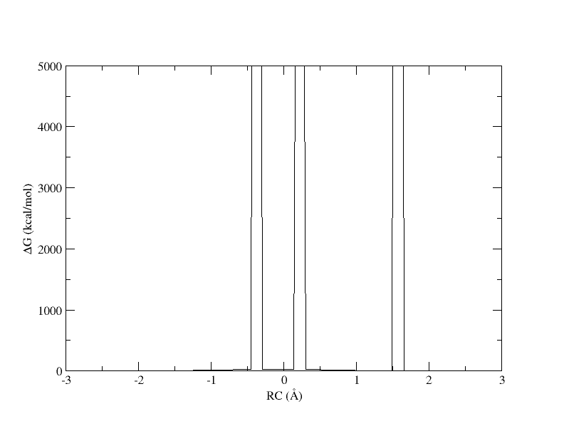
PMF as a function of reaction coordinate value from simulation of 11 umbrella windows analyzed with a 0.15. The free energy is interpolated with 400 spline points. bin width.
The x-axis is the reaction coordinate value and the y-axis is the free energy in kcal/mol. Something has gone horribly wrong and the free energy has shot up to 5000 in 3 places. When we ran the ndfes.OMP command to create the chk file, we used -w 0.15, meaning the bin width when solving the MBAR/UWHAM equations was 0.15 . However, our windows are now spaced ~0.5 apart. In our disang file we set the force constants to be 100 kcal/mol 2. Given our harmonic biasing potential, the distribution of observed reaction coordinates should be approximately normally distributed with a standard deviation of σ=(1/2βK)1/2 where β is the one over the Boltzmann constant times temperature and K is the force constant set in the disang file. Setting rk2 and rk3=100 gives an expected standard deviation in the reaction coordinate of ~0.054 . In a normal distribution, about 99.7% of the samples will be within 3 standard deviations of the mean, which here is ~0.16 . If the windows are ~0.5 away from each other and the sampling spans ~0.16 around the mean, it is highly likely that there will be bins between windows that contain zero samples.
When a bin contains no samples, ndfes reports 5000 for the energy, which effectively indicates it is infinitely high because a calculation could not be made. When we ran ndfes-path.OMP we set –nsplpts to 400 in an attempt to create a smooth spline interpolation through the data, but this meant interpolating through empty bins. Now let’s try running the command again without interpolating. This will just return the free energy at the 11 path points.
Run the following ndfes command:
ndfes-path.OMP --chk metafile.11.0.15.chk --ipath metafile.11 --npathpts 11 --opath path_11_0.5
Plot the result in xmgrace:
xmgrace -block path_11_0.5.rbf.0.dat -bxy 3:4
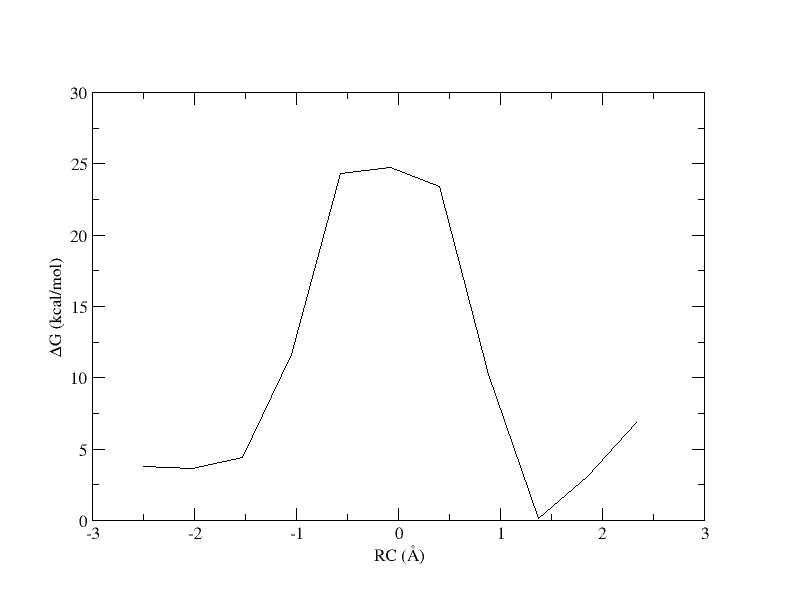
PMF as a function of reaction coordinate value from simulation of 11 umbrella windows analyzed with a 0.15 bin width without spline interpolation.
Now the energy is more reasonable, but the PMF is disjointed. Perhaps is we increase the bin width, there will be no empty bins and we will be able to smoothly interpolate the PMF.
Run the ndfes commands again, but increase the bin width from 0.15 to 0.3 :
ndfes.OMP --mbar -w 0.3 --nboot 0 -c metafile.11.0.3.chk metafile.11
ndfes-path.OMP --chk metafile.11.0.3.chk --ipath metafile.11 --npathpts 11 --nsplpts 400 --opath path_11_spl_0.3
Plot the result in xmgrace:
xmgrace -block path_11_spl_0.3.rbf.0.dat -bxy 3:4
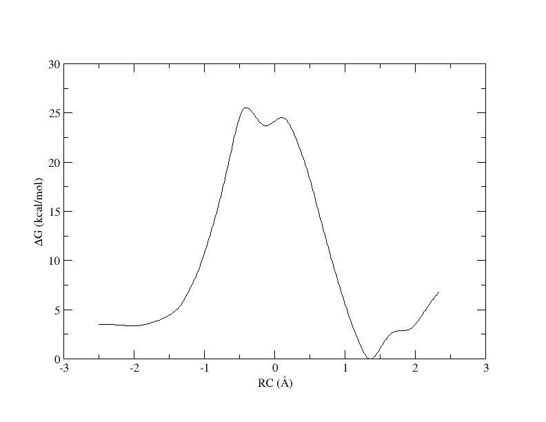
PMF as a function of reaction coordinate value from simulation of 11 umbrella windows analyzed with a 0.3 bin width. The free energy is interpolated with 400 spline points.
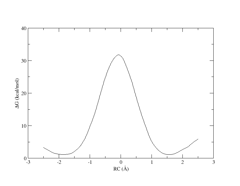
Recall that with 32 windows, the PMF looked like this:
PMF as a function of reaction coordinate value from simulation of all 32 umbrella windows.
As you can see, we were able to make an interpolation, but the PMF is very noisy. All of the bins contain samples, but for many it is not enough to reliably interpolate. In addition, increasing the bin size creates a more course gained view of the free energy landscape. In the end, we simply need more sampling, which is achieved by using more umbrella windows.
The outputs can be downloaded here:
Attention
4.4. References
McCarthy, E.; Ekesan, Ş; Giese, T. J.; Wilson, T. J.; Deng, J.; Huang, L.; Lilley, D. J.; York, D. M. Catalytic mechanism and pH dependence of a methyltransferase ribozyme (MTR1) from computational enzymology. Nucleic Acids Res. 2023, 51, 4508-4518 (10.1093/nar/gkad260)
Giese, T. J.; Ekesan, Ş; York, D. M. Extension of the Variational Free Energy Profile and Multistate Bennett Acceptance Ratio Methods for High-Dimensional Potential of Mean Force Profile Analysis. J. Phys. Chem. A 2021, 125, 4216– 4232 (10.1021/acs.jpca.1c00736)
Gaus, M.; Cui, Q.; Elstner, M. DFTB3: Extension of the Self-Consistent-Charge Density-Functional Tight-Binding Method (SCC-DFTB). J. Chem. Theory Comput. 2011, 7, 931– 948 (10.1021/ct100684s)