3. Hands-On Session 3: Build an RNA enzyme (Ribozyme) containing 12-6-4 divalent ions and non-standard residues
3.1. Learning Objectives
At the end of this hands-on session, you will be able to:
Generate AMBER topology and coordinate files for molecular dynamics simulations
Identify and resolve common atom-type errors encountered during system building
Incorporate non-standard nucleic acid residues using modXNA
Use the RESP procedure to parameterize a non-standard residue
Understand the how discrete MM charges are determined from an electrostatic potential calculation
Learn to use LEaP to solvate an RNA under physiologically relevant conditions
Why do we need a good description of ions–nucleic acids interactions.
Introduce divalent ions described by the 12-6-4 Lennard-Jones potential
Know how to apply 12-6-4 parameters and the PGY pairwise corrections in Amber.
3.2. Relevant literature
McCarthy, E.; Ekesan, Ş.; Giese, T. J.; Wilson, T. J.; Deng, J.; Huang, L.; Lilley, D. J.; York, D. M. Catalytic mechanism and pH dependence of a methyltransferase ribozyme (MTR1) from computational enzymology. Nucleic Acids Research 2023, 51(9), 4508–4518. https://doi.org/10.1093/nar/gkad260
Deng, J.; Wilson, T. J.; Wang, J.; Peng, X.; Li, M.; Lin, X.; Liao, W.; Lilley, D. M. J.; Huang, L. Structure and mechanism of a methyltransferase ribozyme. Nature Chemical Biology 2022, 18(5), 556–564. https://doi.org/10.1038/s41589-022-00982-z
Love, O.; Galindo-Murillo, R.; Roe, D. R.; Dans, P. D.; Cheatham, T. E., III; Bergonzo, C. modXNA: A modular approach to parametrization of modified nucleic acids for use with AMBER force fields. Journal of Chemical Theory and Computation 2024, 20(21), 9354–9363. https://doi.org/10.1021/acs.jctc.4c01164
Bayly, C. I.; Cieplak, P.; Cornell, W.; Kollman, P. A. A well-behaved electrostatic potential based method using charge restraints for deriving atomic charges: the RESP model. J. Phys. Chem. 1993, 97(40), 10269-10280. https://doi.org/10.1021/j100142a004
Panteva, M., Giambasu, G., and York, D. M. Force Field for Mg2+, Mn2+, Zn2+, and Cd2+ Ions That Have Balanced Interactions with Nucleic Acids. J. Phys. Chem. B 2015, 119(50), 15460-15470. https://doi.org/10.1021/acs.jpcb.5b10423
Li, P., and Merz, K. M., Jr. Taking into Account the Ion-Induced Dipole Interaction in the Nonbonded Model of Ions. J. Chem. Theory Comput. 2013, 10(1), 289-297. https://doi.org/10.1021/ct400751u
Zgarbová, M.; Otyepka, M.; Šponer, J.; Mládek, A.; Banáš, P.; Cheatham, T. E., III; Jurečka, P. Refinement of the Cornell et al. nucleic acids force field based on reference quantum chemical calculations of glycosidic torsion profiles. Journal of Chemical Theory and Computation 2011, 7(9), 2886–2902. https://doi.org/10.1021/ct200162x
Horn, H. W.; Swope, W. C.; Pitera, J. W.; Madura, J. D.; Dick, T. J.; Hura, G. L.; Head-Gordon, T. Development of an improved four-site water model for biomolecular simulations: TIP4P-Ew. Journal of Chemical Physics 2004, 120(20), 9665–9678. https://doi.org/10.1063/1.1683075
3.3. Activities
Note
This activity is designed to teach you how to build a system using AMBER and is based on the MTR1 ribozyme that you examined yesterday. However, for pedagogical reasons, the system has been prepared differently here.
The simulations presented yesterday refer to a paper published in 2023, at which time the modXNA parameters (released in 2024) for the parametrization of non-standard residues were not yet available. Therefore, non-standard residues were parametrized using the classical Antechamber and RESP procedure.
In this activity, we will explore both approaches: the classical Antechamber/RESP method (which you will see in more detail later in the context of free energy calculations and ligand parametrization) and the more recent modXNA parametrization.
In addition, for pedagogical purposes, we demonstrate how to apply the Panteva 12-6-4 correction terms for magnesium–nucleic acid interactions. Since no magnesium ions were initially present in the MTR1 structure, the original barium ions were replaced with magnesium ions.
3.3.1. Accessing the activity files
All input files and reference output files required for this activity are provided in two ways.
Option 1: On the cluster
For convenience during the workshop, the full directory associated with Hands-On Session 3 is already available on the cluster and can be copied directly to your working directory from:
/path/Day2/HS3/Files
This directory contains all input files as well as the reference output files corresponding to the preparation of the system. If you have trouble generating a file, you can refer to the files in the input folder or check the output folder.
Option 2: Downloadable archive
All input files and reference output files can also be downloaded as a single compressed archive:
Hands-On Session 3 input and output files (tar.gz)
        flowchart LR

%% ===== access and clean =====
A1["Input files<br/>7v9e.pdb"]
P1{{"<b>[§3.3.1]</b><br/>Access activity files<br/>VMD"}}
P2{{"<b>[§3.3.2]</b><br/>Clean and inspect PDB<br/>pdb4amber"}}
O2["<b>[from §3.3.2]</b><br/>Cleaned structure<br/>7v9e_clean.pdb"]
A1 --> P1
P1 --> P2
P2 --> O2

%% ===== non-standard residues =====
P3{{"<b>[§3.3.3.1]</b><br/>N3-protonated cytidine<br/>modXNA"}}
P4{{"<b>[§3.3.3.2]</b><br/>Restore standard adenine<br/>edit residue"}}
O3["<b>[from §3.3.3]</b><br/>Custom residue libs<br/>lib/frcmod"]
O2 --> P3
O2 --> P4
P3 --> O3
P4 --> O3

%% ===== O6mG ligand parametrization =====
P5{{"<b>[§3.3.3.3.1]</b><br/>Build QM input<br/>Gaussian input"}}
P6{{"<b>[§3.3.3.3.2]</b><br/>Optimize and compute ESP<br/>Gaussian"}}
P7{{"<b>[§3.3.3.3.3]</b><br/>RESP charges and types<br/>antechamber"}}
P8{{"<b>[§3.3.3.3.4]</b><br/>Build parameter files<br/>parmchk2"}}
O4["<b>[from §3.3.3.4]</b><br/>O6mG ligand params<br/>mol2/frcmod"]
P5 --> P6
P6 --> P7
P7 --> P8
P8 --> O4

%% ===== build simulation box =====
P9{{"<b>[§3.3.4.1]</b><br/>Load force fields and residues<br/>tleap"}}
P10{{"<b>[§3.3.4.2]</b><br/>Neutralize with counterions<br/>tleap"}}
P11{{"<b>[§3.3.4.3]</b><br/>Add TIP4P-Ew water<br/>tleap"}}
P12{{"<b>[§3.3.4.4]</b><br/>Add bulk NaCl ions<br/>tleap"}}
O3 --> P9
O4 --> P9
P9 --> P10
P10 --> P11
P11 --> P12

%% ===== Mg 12-6-4 corrections =====
P13{{"<b>[§3.3.5]</b><br/>Apply Mg 12-6-4 PGY corrections<br/>ParmEd"}}
O5["<b>[from §3.3.5]</b><br/>Final system<br/>system.parm7<br/>system.rst7"]
P12 --> P13
P13 --> O5

classDef file fill:#fff7e6,stroke:#d98c00,stroke-width:1.5px,color:#111;
classDef program fill:#e8f1ff,stroke:#1f77b4,stroke-width:1.8px,color:#111;
classDef result fill:#eaf7ea,stroke:#2ca02c,stroke-width:1.5px,color:#111;
class A1 file;
class P1,P2,P3,P4,P5,P6,P7,P8,P9,P10,P11,P12,P13 program;
class O2,O3,O4,O5 result;
3.3.2. Cleaning the PDB file
The inputs should be copied to your working directory. If you unable to produce an output for a given step, copy it from the output directory in order to proceed.
Copy the inputs to your working directory:
[user@cluster] mkdir MTR1_build
[user@cluster] cd MTR1_build
[user@cluster] cp -r /path/Day2/HS3/Files/input/build/* ./
The crystal structure of MTR1 can be obtained from the Protein Data Bank under the ID 7v9e.
Download the structure in PDB file format:
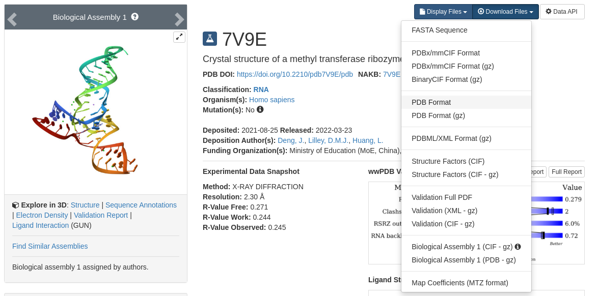
Figure 1. PDB webpage where 7v9e.pdb can be downloaded.
Move this file to your working directory.
You have been provided a set of representations to visualize various aspects of the crystal structure in MTR_crystalreps.txt:
# MTR1 crystal representations

display depthcue off

mol showrep top 0 on

mol selection {all}
mol representation Lines
mol addrep top

# Ions and water (vmd thinks the ligand is solvent, so exclude it)
mol selection {solvent and (not resname GUN)}
mol representation CPK
mol addrep top

# Active site residues
mol selection {resid 10 45 63 101}
mol representation licorice
mol addrep top
Open the pdb file in vmd:
[user@local] vmd 7v9e.pdb
Source the VMD representation file MTR_crystalreps.txt.
In the VMD main window:
Open the Extensions menu
Select Tk Console
In the Tk Console, type:
source MTR_crystalreps.txt
You will see various crystallographic waters and ions that we will ultimately clean from the pdb file before building the system. You will also see that the ribozyme contains two loops and a stem region that meet at a 3 way junction. Junctions are important in RNA structures because they involve bringing the negatively charged phosphates from the backbone close together. This is typically mediated by essential interactions with solvent. Notice that the active site, shown in licorice, is located at the junction.
Hide the rest of the RNA and focus on the active site:
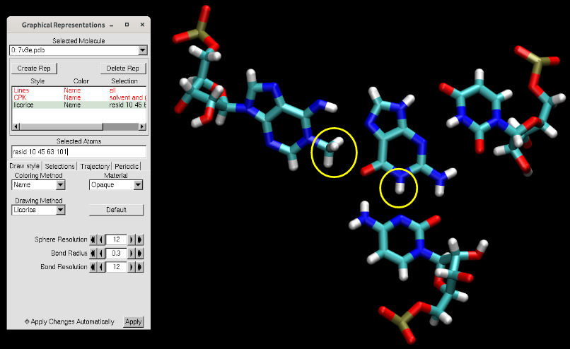
Figure 2. Active site of the MTR1 ribozyme from the crystal structure (PDB ID 7v9e).
This crystal captures the product state of the ribozyme. We see that adenine 63 is methylated at the N1 position. The ribozyme binds O6 methylated guanine to initiate the reaction, so the reactant state would have the methyl group on guanine and a standard adenine for 63. While in the product state N1 of guanine is protonated, the reactant state O6 methylated guanine does not have a proton at N1. We will hypothesize the source of that proton to be N3 position of C10, meaning the reaction starts with C10 protonated with a +1 charge.
Return to your terminal.
PDB files contain many lines giving information about the structure, as well coordinate information for each resolved atom.More information regarding pdb format can be found here. The flags corresponding to atoms and their coordinates, which are the most relevant information for MD simulations, are “ATOM” and “HETATM” where ATOM corresponds main coordinate of the atom, HETATM correspond to coordinates of solvent and ligand atoms not part of the main structure.
Take a look at the PDB file in vim and scroll through to get a sense of the contents.
This pdb file has anisotropic temperature factors reported in ANISOU lines. Since we will have to manually edit some lines in our pdb, we want to work with the minimalist version of the file. We will use the pdb4amber program to achieve that.
We assume you have an AmberTools environment activated, for example:
mamba activate AmberTools25
Run pdb4amber which 7v9e.pdb as input to generate 7v9e_4amber.pdb:
[user@cluster] pdb4amber --in 7v9e.pdb --out 7v9e_4amber.pdb
    ==================================================
    Summary of pdb4amber for: 7v9e.pdb
    ===================================================

    ----------Chains
    The following (original) chains have been found:
    A

    ---------- Alternate Locations (Original Residues!))

    The following residues had alternate locations:
    None
    -----------Non-standard-resnames
    GUN

    ---------- Gaps (Renumbered Residues!)
    gap of 8.021418 A between G 61 and G 63

    ---------- Missing heavy atom(s)

    None
Compare the two pdb files in vmd:
[user@local] vmd -m 7v9e.pdb 7v9e_4amber.pdb
Turn each molecule on and off.
Check that they have the same number of atoms.
Notice that the two structures are indistinguishable. pdb4amber removed introductory lines, ANISOU lines and CONECT lines at the end, and renumbered atoms and residues to be sequential (i.e. residue and/or atom numbers might be different between the two files). Residue 62 (previously 63) is the 1-methyl adenosine, which was not recognized as a standard RNA residue, causing a perceived gap between G 61 and G 63. This is not a problem. Next we will make some manual modifications to our pdb, so let’s first make a new copy to work with.
Copy 7v9e_4amber.pdb to 7v9e_prot.pdb
[user@cluster] cp 7v9e_4amber.pdb 7v9e_prot.pdb
Open 7v9e_prot.pdb in vim.
The remaining REMARK lines would be important for other types of MD simulations such as crystal simulations, but won’t be relevant in this exercise. So if desired they can be removed, but also keeping them will have no effect. The following text blocks have line numbers turned on in vim (:set nu) to help you navigate the file.
Optional: Delete the REMARK lines at the top of the file:
REMARK 290   SMTRY1   1  1.000000  0.000000  0.000000        0.00000
REMARK 290   SMTRY2   1  0.000000  1.000000  0.000000        0.00000
REMARK 290   SMTRY3   1  0.000000  0.000000  1.000000        0.00000
REMARK 290   SMTRY1   2 -1.000000  0.000000  0.000000        0.00000
REMARK 290   SMTRY2   2  0.000000 -1.000000  0.000000        0.00000
REMARK 290   SMTRY3   2  0.000000  0.000000  1.000000       49.96950
REMARK 290   SMTRY1   3 -1.000000  0.000000  0.000000        0.00000
REMARK 290   SMTRY2   3  0.000000  1.000000  0.000000        0.00000
REMARK 290   SMTRY3   3  0.000000  0.000000 -1.000000       49.96950
REMARK 290   SMTRY1   4  1.000000  0.000000  0.000000        0.00000
REMARK 290   SMTRY2   4  0.000000 -1.000000  0.000000        0.00000
REMARK 290   SMTRY3   4  0.000000  0.000000 -1.000000        0.00000
3.3.3. Parametrization of non-standard residues
When working with modified nucleic acids in Amber, non-standard residues are often not available in standard force fields. This activity illustrates two complementary parametrization workflows in Amber using different types of modifications. A protonated cytosine is modeled as a non-standard nucleotide and generated using modXNA. In contrast, O6-methylguanine (O6mG) which is treated as a ligand in the case of MTR1 is therefore parametrized using a traditional RESP and Antechamber approach, as this form is not available in the modXNA library.
3.3.3.1. 2.1 N3-protonated cytidine using modXNA
We would like to “protonate” C10. Since a protonated cytosine is not astandard residue we will use external parameters provided by modXNA. Indeed, modXNA povides a modular, fragment-based framework for building modified nucleotides compatible with modern Amber nucleic acid force fields.
3.3.3.1.1. 2.1.1 Obtaining modXNA
modXNA including the driver script and fragment library, is available on GitHub, through the repository with:
git clone https://github.com/drroe/modXNA.git
This directory contains:
modxna.sh— the main driver scriptdat/— the fragment library (backbone, sugar and base modules)
You should run modxna.sh from within this directory so that the
dat/ folder is found automatically.
modXNA requires AmberTools 25 to be used and available
in the environment. In particular, the following AmberTools components are
used internally:
cpptrajtleap
Make sure AmberTools is properly installed and activated before running
modXNA. For example :
mamba activate AmberTools25
3.3.3.1.2. 2.1.2 modXNA input file
modXNA requires an input text file that specifies which fragments should be assembled to create a modified nucleotide.
Each line of the file follows the format:
<backbone ID> <sugar ID> <base ID>
3.3.3.1.3. 2.1.3 Fragment selection
For this example, we build an RNA residue containing a protonated N3 cytidine. The required fragments are:
RNA backbone:
RPO(standard dimethyl phosphate backbone, charge −1, atom types from OL3)RNA sugar:
RC3(standard ribose sugar in C3′-endo conformation, atom types from OL3)Modified base:
N3C(protonated cystidine in N3, charge +1)
Fragment codes can be checked in the modXNA fragment catalog: https://modxna.chpc.utah.edu/catalog/
3.3.3.1.4. 2.1.4 Creating the input file
Create a text file (for example in-N3C.modxna) with the following content:
### RNA residue with protonated N3 of cytidine
RPO RC3 N3C
3.3.3.1.5. 2.1.5 Running modXNA
Run modXNA using the input file:
 cd modXNA
./modxna.sh -i ../in-N3C.modxna
3.3.3.1.6. 2.1.6 What modXNA does
The program will:
locate the requested fragments in the
dat/directory,remove the capping groups from each fragment,
assemble the backbone, sugar, and base into a single nucleotide,
adjust partial charges to ensure consistency,
perform a short energy minimization to optimize the resulting structure.
When modXNA is run, it automatically assigns a random three-letter name to the newly generated residue. In our example, the residue is named OKC. modXNA produces an OKC.lib file, which can be used to build Amber topology and coordinate files for molecular dynamics simulations.
To incorporate our new residue into our PDB file, we have to rename residue 9 (which corresponds to C10 in the original pdb file before renumbering) from C to OKC (the name of our lib file) and save the PDB file (you can directly modify the 7v9e_prot.pdb).
Warning
When editing PDB files, it is critical to preserve the fixed-column formatting of the PDB standard. Each field must remain within its designated column range; otherwise, errors may occur when building the system in LEaP.
Reminder
The PDB format uses fixed-width columns. Each field must remain within its designated column range; otherwise, errors may occur when building the system in LEaP.
Columns
Column description
1-6
Indicates the
ATOMfield7-11
Atom serial number
13-16
Atom name
17
Alternate location indicator
18-20
Residue name
22
Chain identifier
23-26
Residue sequence number
27
Code for residue insertion
31-38
Orthogonal coordinates for X (Angstrom)
39-46
Orthogonal coordinates for Y (Angstrom)
47-54
Orthogonal coordinates for Z (Angstrom)
55-60
Occupancy
61-66
Temperature factor (B-factor)
77-78
Element symbol
79-80
Atom charge
ATOM    262  P   OKC A   9      18.771   0.638  43.621  1.00 55.52           P
ATOM    263  OP1 OKC A   9      19.026  -0.826  43.656  1.00 74.66           O
ATOM    264  OP2 OKC A   9      19.830   1.583  44.056  1.00 70.25           O
ATOM    265  O5' OKC A   9      18.387   1.029  42.130  1.00 55.31           O
ATOM    266  C5' OKC A   9      17.258   0.451  41.499  1.00 47.08           C
ATOM    267  C4' OKC A   9      16.859   1.235  40.281  1.00 48.52           C
ATOM    268  O4' OKC A   9      16.281   2.504  40.665  1.00 44.83           O
ATOM    269  C3' OKC A   9      18.003   1.628  39.361  1.00 44.20           C
ATOM    270  O3' OKC A   9      18.443   0.567  38.545  1.00 42.92           O
ATOM    271  C2' OKC A   9      17.417   2.801  38.599  1.00 45.04           C
ATOM    272  O2' OKC A   9      16.550   2.358  37.563  1.00 50.64           O
ATOM    273  C1' OKC A   9      16.599   3.485  39.695  1.00 46.71           C
ATOM    274  N1  OKC A   9      17.356   4.568  40.353  1.00 47.41           N
ATOM    275  C2  OKC A   9      17.526   5.751  39.645  1.00 47.12           C
ATOM    276  O2  OKC A   9      17.052   5.815  38.499  1.00 46.70           O
ATOM    277  N3  OKC A   9      18.205   6.764  40.225  1.00 43.87           N
ATOM    278  C4  OKC A   9      18.701   6.624  41.456  1.00 46.67           C
ATOM    279  N4  OKC A   9      19.363   7.668  41.963  1.00 39.22           N
ATOM    280  C5  OKC A   9      18.528   5.423  42.206  1.00 49.00           C
ATOM    281  C6  OKC A   9      17.859   4.425  41.614  1.00 49.69           C
ATOM    282  H5' OKC A   9      16.517   0.434  42.124  1.00 56.60           H
ATOM    283 H5'' OKC A   9      17.470  -0.459  41.237  1.00 56.60           H
ATOM    284  H4' OKC A   9      16.194   0.731  39.786  1.00 58.32           H
ATOM    285  H3' OKC A   9      18.752   1.941  39.891  1.00 53.14           H
ATOM    286  H2' OKC A   9      18.103   3.391  38.250  1.00 54.15           H
ATOM    287 HO2' OKC A   9      16.855   2.616  36.823  1.00 60.87           H
ATOM    288  H1' OKC A   9      15.781   3.844  39.317  1.00 56.16           H
ATOM    289  H41 OKC A   9      19.699   7.621  42.753  1.00 47.16           H
ATOM    290  H42 OKC A   9      19.452   8.387  41.500  1.00 47.16           H
ATOM    291  H5  OKC A   9      18.866   5.336  43.069  1.00 58.90           H
ATOM    292  H6  OKC A   9      17.735   3.623  42.068  1.00 59.73           H
3.3.3.2. 2.2 From the methylated adenine to a standard one
Next we will “mutate” the methylated adenine, 1MA, back to a standard adenine. This requires changing residue name from 1MA to A, and deleting the methyl atoms. We’ll start with deleting the atoms so we have less atoms to rename residue names of.
Delete methyl atoms and additional hydrogen of residue number 62 (A63 in the original pdb file before renumbering): CM1, HN61, HM11, HM12, and HM13.
Change the residue name of 62 from 1MA to A, by changing 1 to A, and changing M and A into two empty spaces, so that the total number of columns is not modified:
ATOM   1946  P   A   A  62      22.724  23.209  43.994  1.00 70.56           P
ATOM   1947  OP1 A   A  62      23.291  23.505  45.361  1.00 73.73           O
ATOM   1948  OP2 A   A  62      23.176  24.033  42.821  1.00 88.65           O
ATOM   1949  O5' A   A  62      22.969  21.684  43.646  1.00 63.06           O
ATOM   1950  C5' A   A  62      24.006  20.974  44.301  1.00 68.95           C
ATOM   1951  C4' A   A  62      23.489  20.121  45.431  1.00 58.78           C
ATOM   1952  O4' A   A  62      22.595  19.115  44.876  1.00 60.31           O
ATOM   1953  C3' A   A  62      24.569  19.343  46.178  1.00 56.81           C
ATOM   1954  O3' A   A  62      24.128  19.101  47.511  1.00 55.15           O
ATOM   1955  C2' A   A  62      24.610  18.029  45.411  1.00 51.57           C
ATOM   1956  O2' A   A  62      25.177  16.949  46.126  1.00 52.34           O
ATOM   1957  C1' A   A  62      23.117  17.826  45.125  1.00 54.19           C
ATOM   1958  N9  A   A  62      22.827  16.957  43.975  1.00 54.44           N
ATOM   1959  C8  A   A  62      23.376  17.668  42.954  1.00 52.77           C
ATOM   1960  N7  A   A  62      23.192  16.958  41.807  1.00 40.69           N
ATOM   1961  C5  A   A  62      22.523  15.840  42.134  1.00 45.39           C
ATOM   1962  C6  A   A  62      22.012  14.634  41.321  1.00 49.52           C
ATOM   1963  N6  A   A  62      22.234  14.614  40.078  1.00 44.46           N
ATOM   1964  N1  A   A  62      21.313  13.559  41.983  1.00 45.82           N
ATOM   1966  C2  A   A  62      21.087  13.586  43.394  1.00 45.05           C
ATOM   1967  N3  A   A  62      21.577  14.723  44.151  1.00 48.62           N
ATOM   1968  C4  A   A  62      22.304  15.843  43.481  1.00 49.84           C
ATOM   1969  H5' A   A  62      24.644  21.612  44.658  1.00 82.84           H
ATOM   1970 H5'' A   A  62      24.449  20.402  43.655  1.00 82.84           H
ATOM   1971  H4' A   A  62      22.998  20.672  46.060  1.00 70.64           H
ATOM   1972  H3' A   A  62      25.426  19.797  46.154  1.00 68.27           H
ATOM   1973  H2' A   A  62      25.087  18.142  44.574  1.00 61.99           H
ATOM   1974 HO2' A   A  62      25.201  17.142  46.957  1.00 62.91           H
ATOM   1975  H1' A   A  62      22.686  17.458  45.912  1.00 65.13           H
ATOM   1976  H8  A   A  62      23.815  18.352  42.502  1.00 63.43           H
ATOM   1981  H2  A   A  62      20.636  12.891  43.817  1.00 54.16           H
3.3.3.3. 2.3 Parametrization of the ligand, O6 methylguanine (O6mG)
We next considered the ligand (residue name GUN). Although O6-methylated guanine is available in modXNA, that implementation assumes the presence of a nucleic-acid backbone and sugar. In our case, the ligand consists solely of the base capped with a hydrogen atom; therefore, we have to use the standard parametrization approach for non-standard residues.
You will utilize antechamber to determine atom types carry out the restrained electrostatic potential (RESP) procedure to obtain partial charges for the non-standard residue GUN, O6 methylated guanine ligand), and build parameter files. You will go through the following sections:
2.3.1 Preparing a Gaussian input file
2.3.2 Structure optimization and ESP charges with Gaussian
2.3.3 Atom types and partial charges using antechamber and RESP procedure
2.3.4 Building parameter files
3.3.3.3.1. 2.3.1 Preparing a Gaussian input file
AMBER residue parameters are defined by atom types and partial charges. AMBER has a wide list of atom types with established MM parameters regarding bond lengths, angles, dihedral angles and vdW radii. Partial charges that go into the electrostatics calculation of the force are described separately. So generating parameters for a new residue requires atom type selection and partial charge determination.
In this section you will see how a Gaussian input file was created using GaussView based on the ligand structure in the pdb file. If you have GaussView available to you, feel free to attempt this section. Otherwise, follow along to see what actions were taken. You have been provided a pdb file of the ligand that was present in the crystal structure in the product state. We will need to edit this structure to be in the reactant state.
The following steps were taken to prepare a Gaussian input file for O6 methylated guanine based on the crystal structure coordinates of the guanine product in the crystal. Recall that the methyl group had already been transferred from the ligand.
GUN.pdb was opened with GaussView.
GUN.pdb
A methyl group was added to the oxygen, and the hydrogen that we put on C10 in the previous section was deleted.
[user@local] gv GUN.pdb
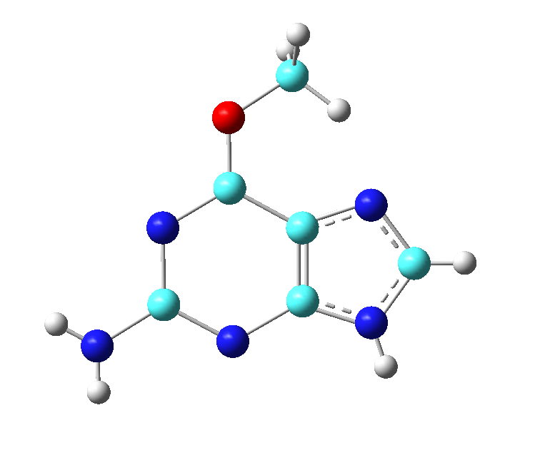
Figure 1. Structure of O6 methylated guanine that was edited with GaussView.
The structure was saved as a Gaussian input file called GUN.gjf, which is provided for you in the inputs.
The input file would look something like this:
%chk=GUN.chk
# hf/3-21g

Title Card Required

0 1
 N                 20.05213100   11.86058800   36.02351400
 C                 20.78663800   12.65045600   36.89290400
 N                 20.90570600   12.13218500   38.09712300
 C                 20.20665200   10.92676800   38.02243900
 C                 19.93136600    9.86610100   38.92113800
 O                 20.33478900    9.77794100   40.20264300
 N                 19.21047500    8.81736400   38.51825700
 C                 18.75247500    8.79396500   37.24439200
 N                 17.96142200    7.71264700   36.91957400
 N                 18.94068400    9.71428900   36.27043500
 C                 19.66323200   10.73955800   36.72590700
 H                 19.82722600   12.05265800   35.05295000
 H                 21.20875900   13.60185700   36.57547400
 H                 17.88964300    7.52051800   35.92518000
 H                 18.08578800    6.90435000   37.52121100
 C                 21.11877500   10.85660800   40.73877700
 H                 20.56584100   11.80695700   40.70657800
 H                 21.32467200   10.57091700   41.77831600
 H                 22.06005100   10.98164000   40.18349700
3.3.3.3.2. 2.3.2 Structure optimization and ESP charges with Gaussian
In this section you will build and optimize the ligand structure and calculate corresponding electrostatic potential (ESP) charges using Gaussian in order to generating non-standard residue parameters. You will generate parameters for the non-standard O6 methylated guanine ligand using the restrained electrostatic potential (RESP) procedure. The input file was edited to run an optimization of the structure and an electrostatic potential (ESP) calculation. The optimization will be done at a high level of DFT, and the ESP will be computed at the Hartree Fock level to be consistent with the methods used to generate the standard AMBER charges.
The input file provided should look as follows:
%chk=GUN.chk
%nprocshared=4
%mem=10GB
# opt pbepbe/6-31g(2d,2p)

GUN_opt

0 1
 N                 20.05213100   11.86058800   36.02351400
 C                 20.78663800   12.65045600   36.89290400
 N                 20.90570600   12.13218500   38.09712300
 C                 20.20665200   10.92676800   38.02243900
 C                 19.93136600    9.86610100   38.92113800
 O                 20.33478900    9.77794100   40.20264300
 N                 19.21047500    8.81736400   38.51825700
 C                 18.75247500    8.79396500   37.24439200
 N                 17.96142200    7.71264700   36.91957400
 N                 18.94068400    9.71428900   36.27043500
 C                 19.66323200   10.73955800   36.72590700
 H                 19.82722600   12.05265800   35.05295000
 H                 21.20875900   13.60185700   36.57547400
 H                 17.88964300    7.52051800   35.92518000
 H                 18.08578800    6.90435000   37.52121100
 C                 21.11877500   10.85660800   40.73877700
 H                 20.56584100   11.80695700   40.70657800
 H                 21.32467200   10.57091700   41.77831600
 H                 22.06005100   10.98164000   40.18349700

--link1--

%chk=GUN.chk
%nprocshared=4
%mem=10GB
#P HF/6-31G* SCF(Conver=6) NoSymm Test Pop=mk IOp(6/33=2) guess=read geom=allcheck GFInput GFPrint
Make sure there is a blank line at the end of the file.
The first section indicates the optimization, and the link uses the optimized structure to calculate the ESP. The ESP will be represented on a grid of points. The keyword IOp(6/33=2) instructs Gaussian to output this information for use later when performing the RESP fit. You have also been provided a file called gau.slurm to run the job on expanse.
Submit the job:
[user@cluster] sbatch gau.slurm
For time constraints, you will be able to review the result once the calculation is complete. We nevertheless provide the remainder so that you can continue. When the job is finished, make sure the last line of GUN.log reports “Normal termination of Gaussian”.
3.3.3.3.3. 2.3.3 Atom types and partial charges using antechamber and RESP procedure
Next we will use the antechamber program to assign point charges based on the ESP. The fit will be performed such that topologically equivalent atoms have the same charge.
Run the following antechamber command to use the ESP to assign charges using the RESP procedure:
[user@cluster] antechamber -i GUN.log -fi gout -o GUN.mol2 -fo mol2 -c resp -at gaff -pf y -rn GUN
This will create GUN.mol2. We used the flag -c resp to read the ESP from the Gaussian output file and perform RESP. The -at gaff flag means atoms types are assigned from the GAFF force field, -pf y removes intermediate files, and -rn GUN sets the residue name in the mol2 file to be GUN. This is the name we used in the PDB file when building the system.
Take a look at GUN.mol2:
@<TRIPOS>MOLECULE
GUN
19 20 1 0 0
SMALL
resp
@<TRIPOS>ATOM
1 N1 20.0520 11.8610 36.0240 na 1 GUN -0.334523
2 C1 20.7870 12.6500 36.8930 cc 1 GUN 0.097034
3 N2 20.9060 12.1320 38.0970 nd 1 GUN -0.523097
4 C2 20.2070 10.9270 38.0220 ca 1 GUN 0.144003
5 C3 19.9310 9.8660 38.9210 ca 1 GUN 0.558035
6 O1 20.3350 9.7780 40.2030 os 1 GUN -0.329698
7 N3 19.2100 8.8170 38.5180 nb 1 GUN -0.745822
8 C4 18.7520 8.7940 37.2440 ca 1 GUN 0.884237
9 N4 17.9610 7.7130 36.9200 nh 1 GUN -0.890772
10 N5 18.9410 9.7140 36.2700 nb 1 GUN -0.693379
11 C5 19.6630 10.7400 36.7260 ca 1 GUN 0.325075
12 H1 19.8270 12.0530 35.0530 hn 1 GUN 0.347262
13 H2 21.2090 13.6020 36.5750 h5 1 GUN 0.176097
14 H3 17.8900 7.5210 35.9250 hn 1 GUN 0.381855
15 H4 18.0860 6.9040 37.5210 hn 1 GUN 0.381855
16 C6 21.1190 10.8570 40.7390 c3 1 GUN -0.005320
17 H5 20.5660 11.8070 40.7070 h1 1 GUN 0.075719
18 H6 21.3250 10.5710 41.7780 h1 1 GUN 0.075719
19 H7 22.0600 10.9820 40.1830 h1 1 GUN 0.075719
@<TRIPOS>BOND
1 1 2 1
2 1 11 1
3 1 12 1
4 2 3 2
5 2 13 1
6 3 4 1
7 4 5 ar
8 4 11 ar
9 5 6 1
10 5 7 ar
11 6 16 1
12 7 8 ar
13 8 9 1
14 8 10 ar
15 9 14 1
16 9 15 1
17 10 11 ar
18 16 17 1
19 16 18 1
20 16 19 1
@<TRIPOS>SUBSTRUCTURE
1 GUN 1 TEMP 0 **** **** 0 ROOT
The mol2 file contains the point charges and atom types. For example, notice that the methyl group hydrogen atoms (H5,H6, and H7) were all assigned the same charge because they are topologically equivalent. When fitting was performed, it would have been done under the constraint that these should have the same charge. Similarly, the amine hydrogens (H3 and H4) are also equivalent.
Test to make sure the charges in the mol2 file approximately sum to zero by extracting them from the mol2 file.
[user@cluster] sed -n -e '9,27p' GUN.mol2 | awk '{print $9}' > charges.dat
[user@cluster] cat charges.dat
-0.334523
0.097034
-0.523097
0.144003
0.558035
-0.329698
-0.745822
0.884237
-0.890772
-0.693379
0.325075
0.347262
0.176097
0.381855
0.381855
-0.005320
0.075719
0.075719
0.075719

[user@cluster] awk '{ sum += $1 } END { print sum }' charges.dat
-1e-06
3.3.3.3.4. 2.3.4 Building parameter files
Now we must create parameter files that are compatible with AMBER.
Use tleap to generate a .lib file containing the charges determined from RESP:
cat << EOF > tleap_GUN.in

source leaprc.gaff
GUN = loadmol2 GUN.mol2
SaveOff GUN GUN.lib
saveamberparm GUN GUN.parm7 GUN.rst7
quit

EOF

tleap -sf tleap_GUN.in
tleap_GUN.in
GUN.lib
GUN.parm7
GUN.rst7
We will determine the geometric parameters from the GAFF force field. Each atom in the parameter file has been assigned a type from the GAFF force field, so we will search the existing library of parameters for these atom type.
Use parmed to write geometric parameters to the frcmod file.
cat << EOF > parmed_GUN.in

parm GUN.parm7
loadRestrt GUN.rst7
writeFrcmod GUN.frcmod
quit

EOF

parmed -i parmed_GUN.in
Note
Now you have all parameter files required to build and run the MTR1 system, the protonated cytosine, and the methylated guanine.
3.3.3.4. 2.4 Finalization of system preparation
The atom names reported in the pdb are different than atom names we have in our parameter file.
Print the atom types in GUN.lib:
[user@cluster] head -n22 GUN.lib
!!index array str
 "GUN"
!entry.GUN.unit.atoms table  str name  str type  int typex  int resx  int flags  int seq  int elmnt  dbl chg
 "N1" "na" 0 1 131072 1 7 -0.334523
 "C1" "cc" 0 1 131072 2 6 0.097034
 "N2" "nd" 0 1 131072 3 7 -0.523097
 "C2" "ca" 0 1 131072 4 6 0.144003
 "C3" "ca" 0 1 131072 5 6 0.558035
 "O1" "os" 0 1 131072 6 8 -0.329698
 "N3" "nb" 0 1 131072 7 7 -0.745822
 "C4" "ca" 0 1 131072 8 6 0.884237
 "N4" "nh" 0 1 131072 9 7 -0.890772
 "N5" "nb" 0 1 131072 10 7 -0.693379
 "C5" "ca" 0 1 131072 11 6 0.325075
 "H1" "hn" 0 1 131072 12 1 0.347262
 "H2" "h5" 0 1 131072 13 1 0.176097
 "H3" "hn" 0 1 131072 14 1 0.381855
 "H4" "hn" 0 1 131072 15 1 0.381855
 "C6" "c3" 0 1 131072 16 6 -0.005320
 "H5" "h1" 0 1 131072 17 1 0.075719
 "H6" "h1" 0 1 131072 18 1 0.075719
 "H7" "h1" 0 1 131072 19 1 0.075719
We need to rename the heavy atoms in the pdb file 7v9e_prot.pdb to their corresponding names in the parameter file. In order to simplify this process we will first remove the protons within the residue. LEaP can easily add these back later with the correct names.
Delete the protons HN1, HN9, H8, HN21, and HN22.
Rename the heavy atoms atoms as follows:
HETATM 2175  N1  GUN A  69      20.435  11.931  36.172  1.00 40.72           N
HETATM 2176  C1  GUN A  69      21.059  12.713  37.080  1.00 45.85           C
HETATM 2177  N2  GUN A  69      21.000  12.094  38.277  1.00 37.65           N
HETATM 2178  C2  GUN A  69      20.352  10.944  38.115  1.00 42.37           C
HETATM 2179  C3  GUN A  69      19.965   9.819  39.086  1.00 43.44           C
HETATM 2180  O1  GUN A  69      20.255   9.900  40.233  1.00 39.68           O
HETATM 2181  N3  GUN A  69      19.246   8.676  38.614  1.00 43.96           N
HETATM 2182  C4  GUN A  69      18.873   8.588  37.236  1.00 43.78           C
HETATM 2183  N4  GUN A  69      18.150   7.445  36.734  1.00 40.36           N
HETATM 2184  N5  GUN A  69      19.248   9.652  36.333  1.00 41.19           N
HETATM 2185  C5  GUN A  69      19.996  10.845  36.806  1.00 45.72           C
Barium and sodium ions, together with a small number of water molecules, were resolved crystallographically. These species are not catalytically relevant. For this reason, sodium ions and crystallographic water molecules were removed. The barium ions were intentionally retained and subsequently replaced by magnesium ions in order to illustrate in practice how 12-6-4 Lennard-Jones correction terms with Panteva–Giambasu–York (PGY) pairwise correcions are applied, enabling balanced interactions with nucleic acids.
Delete sodium ion and water molecules.
HETATM 2200 NA   NA  A  79      36.287  16.215  43.272  1.00 34.26          NA
HETATM 2201 NA   NA  A  80      31.896   7.690  34.088  1.00 50.91          NA
HETATM 2202  O   HOH A  81      43.549  22.559  52.718  1.00 67.88           O
HETATM 2203  O   HOH A  82      46.224  26.856  56.524  1.00 69.56           O
HETATM 2204  O   HOH A  83      -0.607  23.932  34.220  1.00 62.80           O
HETATM 2205  O   HOH A  84      13.884  27.718  35.721  1.00 64.85           O
HETATM 2206  O   HOH A  85      15.463   4.299  36.801  1.00 47.72           O
HETATM 2207  O   HOH A  86       8.577  12.465  25.488  1.00 70.15           O
HETATM 2208  O   HOH A  87      27.735  18.894  46.490  1.00 40.64           O
HETATM 2209  O   HOH A  88      33.130  -4.678  33.799  1.00 32.49           O
HETATM 2210  O   HOH A  89      32.100   4.191  32.161  1.00 39.50           O
HETATM 2211  O   HOH A  90      26.286   0.200  32.199  1.00 50.23           O
HETATM 2212  O   HOH A  91      36.070  10.612  25.896  1.00 55.39           O
HETATM 2213  O   HOH A  92      25.235  17.366  32.641  1.00 57.43           O
HETATM 2214  O   HOH A  93      34.079 -14.419  28.448  1.00 52.99           O
HETATM 2215  O   HOH A  94      35.911  -4.317  32.231  1.00 33.16           O
HETATM 2216  O   HOH A  95      28.622  -6.340  30.512  1.00 55.39           O
HETATM 2217  O   HOH A  96      21.541  18.363  31.228  1.00 45.76           O
HETATM 2218  O   HOH A  97      39.960   0.108  40.497  1.00 46.79           O
HETATM 2219  O   HOH A  98       5.321  31.207  42.190  1.00 59.35           O
HETATM 2220  O   HOH A  99      -0.444  19.583  36.126  1.00 52.16           O
HETATM 2221  O   HOH A 100      28.698   0.541  51.368  1.00 59.76           O
HETATM 2222  O   HOH A 101      15.735  -0.430  36.539  1.00 55.39           O
HETATM 2223  O   HOH A 102      37.524   9.301  27.209  1.00 62.05           O
HETATM 2224  O   HOH A 103      28.598  21.370  47.356  1.00 48.57           O
HETATM 2225  O   HOH A 104      33.224   6.071  32.685  1.00 44.69           O
HETATM 2226  O   HOH A 105      28.951  21.487  44.742  1.00 56.37           O
HETATM 2227  O   HOH A 106      30.511  21.905  41.786  1.00 63.69           O
HETATM 2228  O   HOH A 107      33.481  24.017  45.493  1.00 47.89           O
HETATM 2229  O   HOH A 108      -3.444  23.781  35.501  1.00 60.89           O
HETATM 2230  O   HOH A 109      27.024  21.879  45.193  1.00 58.85           O
HETATM 2231  O   HOH A 110      32.792  -2.728  32.364  1.00 43.28           O
HETATM 2232  O   HOH A 111      30.418  23.355  48.435  1.00 55.87           O
HETATM 2233  O   HOH A 112      31.672  27.219  56.474  1.00 56.58           O
And then, replace barium ions by magnesium ions.
HETATM 2191 MG   MG  A  70      31.906   8.390  45.892  0.60 24.18          MG
HETATM 2192 MG   MG  A  71      34.813  -6.355  31.778  0.58 30.39          MG
HETATM 2193 MG   MG  A  72      31.033   0.308  49.682  0.40 61.24          MG
HETATM 2194 MG   MG  A  73      33.004  17.329  49.683  0.45 54.07          MG
HETATM 2195 MG   MG  A  74      27.824  -1.912  53.472  0.40 46.29          MG
HETATM 2196 MG   MG  A  75      32.282  24.572  53.839  0.48 69.02          MG
HETATM 2197 MG   MG  A  76       0.279  22.083  36.141  0.75 84.35          MG
HETATM 2198 MG   MG  A  77      18.560  14.938  32.414  0.56 62.27          MG
HETATM 2199 MG   MG  A  78       8.384  17.597  38.313  0.76120.11          MG
Save and close the pdb file.
Visually inspect the structure in vmd to ensure you have made the desired changes.
Source MTR_cleanreps.txt:
# MTR1 clean pdb representations

display depthcue off

mol showrep top 0 on

# Ions and water (vmd thinks the ligand is solvent, so exclude it)
mol selection {solvent and (not resname GUN)}
mol representation CPK
mol addrep top

# Active site residues
mol selection {resid 9 44 62 69}
mol representation licorice
mol addrep top
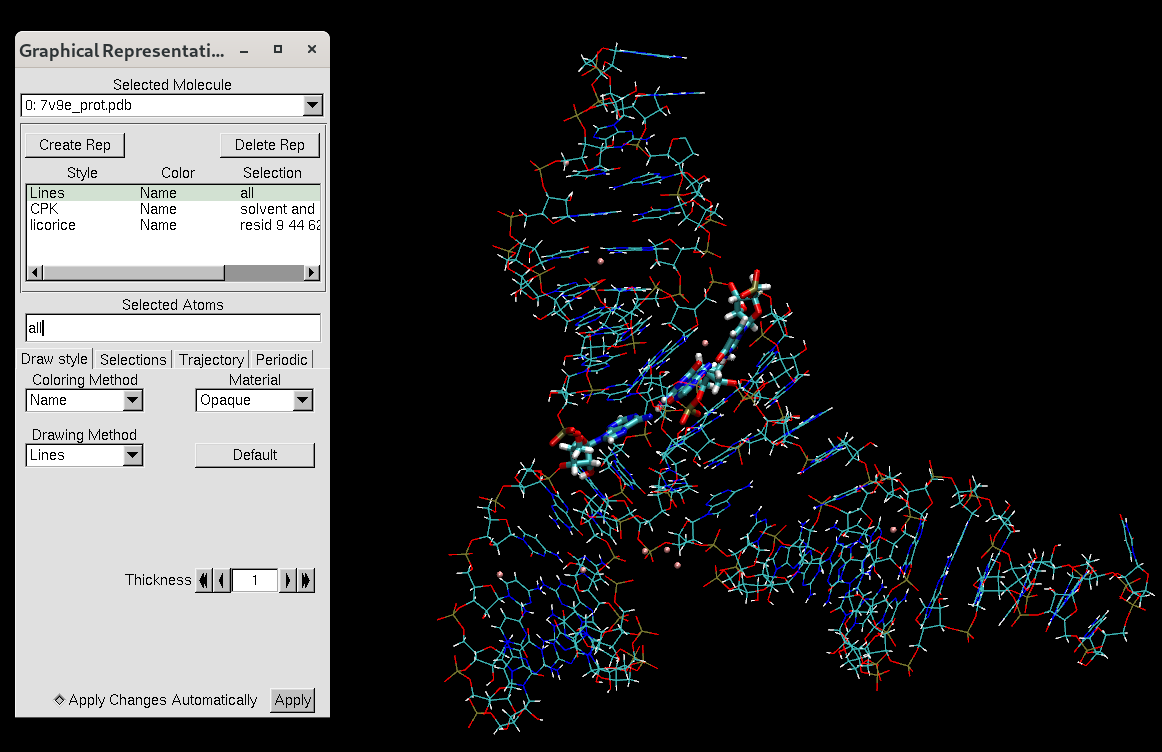
Figure 3. VMD representation of the MTR1 ribozyme after editing the PDB file.
There should be no solvent remaining but you could see the magnesium ions. Since the pdb file has been reordered, the active site residues have different numbers from the file we downloaded from the PDB website. The active site representation now contains residues 9, 44, 62, and 69, which used to be residues 10, 45, 63, and 101.
Source MTR_cleanreps.txt again to use the representations.
Hide all and focus on the active site in licorice.
Select some of the active site atoms to confirm that the residue names have been changed.
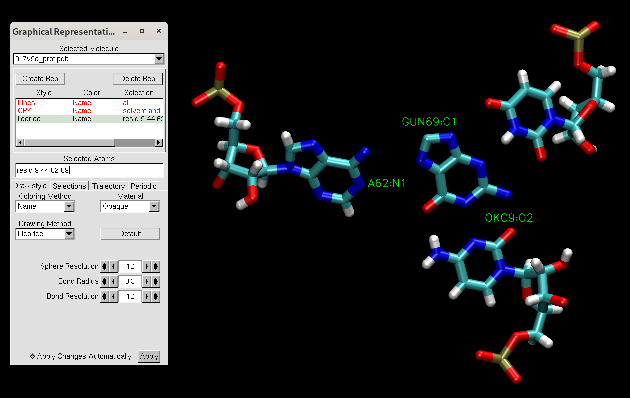
Figure 4. VMD representation of the MTR1 active site after editing the PDB file.
3.3.4. Building the Simulation Box
AMBER has a program named LEaP, which takes in coordinates and force field definitions and produces parameter and restart files needed for system definition by the MD engine. We will use LEaP to create a simulation box that has explicit water molecules, Na+, Cl- and Mg2+ ions, as well as our RNA-ligand system in its protonated state. This process is also referred to as “solvating the system”. LEaP can fill in missing atoms, but it will not delete atoms. This means the structure cannot contain atom types not included in a force field.
LEaP has a specific order of events. Force field parameters need to be loaded first, followed by loading the molecule. Next solvent and ions are added and finally output files need to be saved. Nucleic acids benefit from adding ions and water in a specific order. For pedagogical reasons, we will start with a step-wise approach to building the simulation box. At the end we will have a single input file that will build the simulation box in one go.
3.3.4.1. 3.1 Force fields and loading the molecule
In order for a molecule to be loaded without error, every residue and atom in the input structure must have a corresponding parameter set already loaded in LEaP. AMBER provides a variety of well-established force fields for proteins and nucleic acids, as well as water models and metal ion parameters. The current recommendation for RNA simulations is the OL3 force field (Zgarbová, 2011).
We use the TIP4P-Ew water model (Horn, 2004) for nucleic acid systems due to the availability of fine-tuned ion parameters compatible – which are often critical for nucleic acid structure and function – including 12-6-4 Lennard-Jones corrections for monovalent ions (Sengupta, 2021). For Mg2+ ions, Panteva–Giambasu–York (PGY) pairwise corrections are applied in conjunction with the 12-6-4 model to improve the description of RNA–magnesium interactions (Panteva, 2015).
Additionally, our system contains two non-standard residues (i.e. residue names not readily available in the standard AMBER force fields), which have been newly parameterized. The corresponding parameter files are provided as OKC.lib, GUN.lib, and GUN.frcmod.
First, we verify that all required definitions are correctly loaded by building the topology and restart files for the RNA–ligand system alone, without any solvent.
Take a look at tleap_MTR1_param.in
set default nocenter on # Do not recenter the molecule

### Sourcing amber forcefields ###############################################

source leaprc.RNA.OL3 # Sourcing RNA force field OL3 to describe RNA.
source leaprc.water.tip4pew # Sourcing water model TIP4P-Ew
                            # and parameters for corresponding monovalent ions
#loadamberparams frcmod.ions234lm_1264_tip4pew # divalent metal ion parameters

### Including non-standard residue parameters ################################

# Ligand O6 methylated guanine
loadoff GUN.lib
loadamberparams GUN.frcmod

# N3 protonated cytosine
loadoff OKC.lib
loadamberparams ./modXNA/dat/frcmod.modxna

### Loading structure from file ##############################################
mol= loadpdb "7v9e_prot.pdb"

### Saving output files  #####################################################
# save parameter and restart files
saveamberparm mol MTR1_noSolvent.parm7 MTR1_noSolvent.rst7
quit
Run tleap with tleap_MTR1_param.in as input:
[user@cluster] tleap -sf tleap_MTR1_param.in
For pedagogical reasons, we intentionally left the following error:
FATAL:  Atom .R<C5 1>.A<P 30> does not have a type.
FATAL:  Atom .R<C5 1>.A<OP1 31> does not have a type.
FATAL:  Atom .R<C5 1>.A<OP2 32> does not have a type.
These errors indicate that phosphate atoms are present at the 5’ end of the nucleic acid chain, which is incompatible with AMBER’s residue definitions. In AMBER, 5’ and 3’ terminal residues are treated differently: the 5’ end is capped at the O5’ atom, and this capping requires the absence of phosphate groups.
To fix this problem, the phosphate group must be removed from the 5’ terminal residue (residue 1). Since this involves modifying the structure file, we first create a copy of the original PDB file to preserve it.
Copy the file 7v9e_prot.pdb to a new file named 7v9e_C5.pdb. All subsequent modifications to correct the error will be performed on this new file.
cp 7v9e_prot.pdb 7v9e_C5.pdb
Delete the phosphate atoms (P, OP1, and OP2) from residue 1 in 7v9e_C5.pdb, as shown below:
ATOM      1  P   C   A   1      36.782  21.325  44.826  1.00 96.64           P
ATOM      2  OP1 C   A   1      36.892  20.457  43.625  1.00 89.80           O
ATOM      3  OP2 C   A   1      35.628  21.157  45.749  1.00 78.55           O
Then, you can define a new input file for tleap, with this new pdb.
Take a look at tleap_MTR1_param_C5.in
set default nocenter on # Do not recenter the molecule

### Sourcing amber forcefields ###############################################

source leaprc.RNA.OL3 # Sourcing RNA force field OL3 to describe RNA.
source leaprc.water.tip4pew # Sourcing water model TIP4P-Ew
                            # and parameters for corresponding monovalent ions
#loadamberparams frcmod.ions234lm_1264_tip4pew # divalent metal ion parameters

### Including non-standard residue parameters ################################

# Ligand O6 methylated guanine
loadoff GUN.lib
loadamberparams GUN.frcmod

# N3 protonated cytosine
loadoff OKC.lib
loadamberparams ./modXNA/dat/frcmod.modxna

### Loading structure from file ##############################################
mol= loadpdb "7v9e_C5.pdb"  #UPDATED PDB

### Saving output files  #####################################################
# save parameter and restart files
saveamberparm mol MTR1_noSolvent.parm7 MTR1_noSolvent.rst7
quit
Run tleap with tleap_MTR1_param_C5.in as input:
[user@cluster] tleap -sf tleap_MTR1_param_C5.in
Visualize the resulting parameter and restart file in vmd. You may continue to use the MTR_cleanreps.txt until otherwise specified.
[user@local] vmd MTR1_noSolvent.parm7 MTR1_noSolvent.rst7
Hide all and focus on the active site.
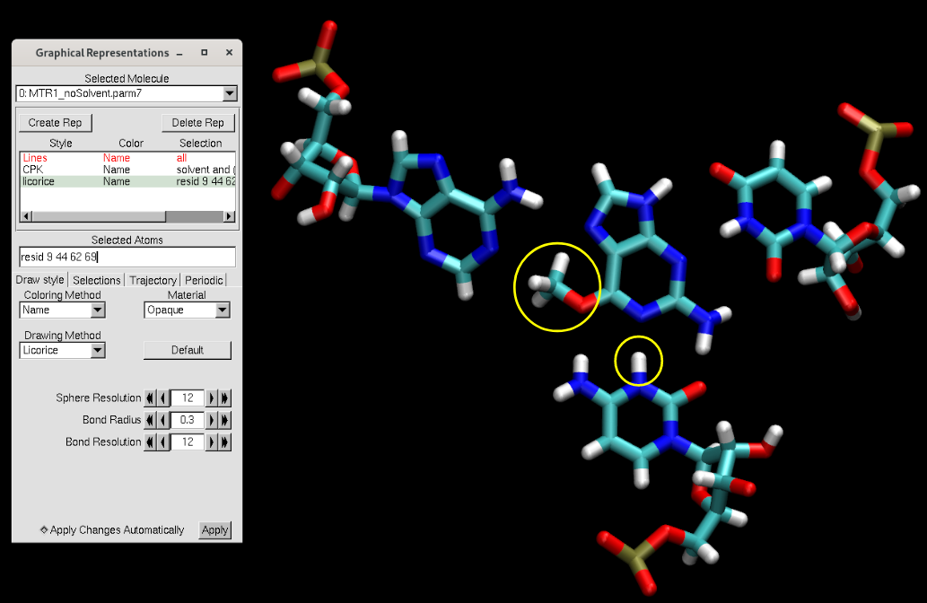
Figure 5. VMD representation of the MTR1 active site after adding missing atoms with LEaP.
You will see that the methyl group was added on the ligand, and a proton was added onto the cytosine (circled in yellow above). Additionally, missing hydrogen atoms were added.
3.3.4.2. 3.2 Neutralize the system with counterions
Now we will only add the counter ions to our system. Use the tleap_MTR1_counterIon.in input file, which differs from the above by only the inclusion of the following line and output file names.
### Adding counter ions ######################################################
addions mol NA 0 # Add sodium until charge is zero
Run tleap with the following command:
[user@cluster] tleap -f tleap_MTR1_counterIon.in
Visualize the output structures in vmd
[user@local] vmd MTR1_counterIon.parm7 MTR1_counterIon.rst7
MTR1_counterIon.parm7
MTR1_counterIon.rst7
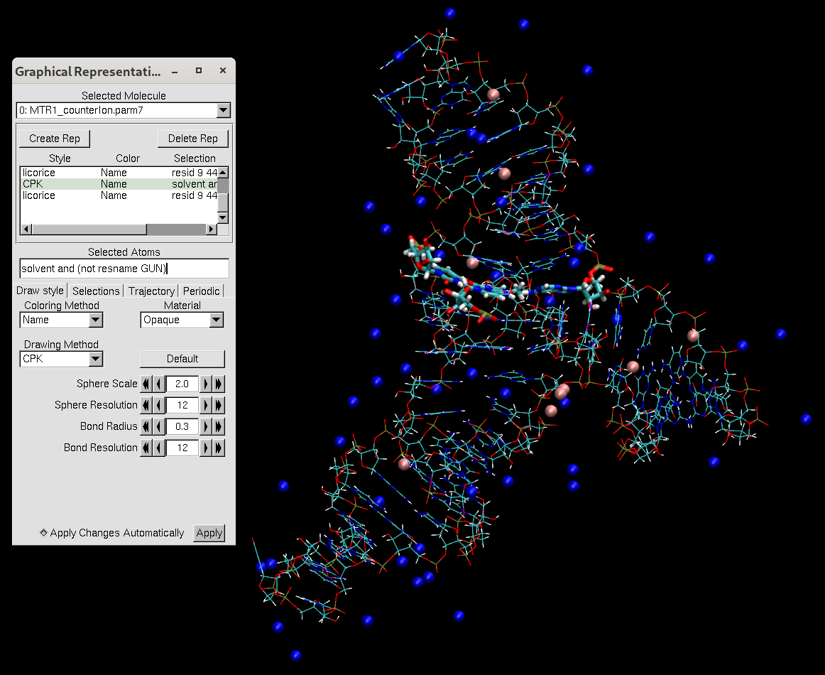
Figure 6. VMD representation of the MTR1 ribozyme after adding counter ions.
You will notice that the counterions are placed along the phosphate backbone, which is negatively charged. It is essential to neutralize the backbone to stabilize the structure. We add the counterions before adding water to avoid the ions being placed far away from the RNA.
3.3.4.3. 3.3 Add water molecules
Next we will add water molecules. The simulations will ultimately take place under periodic boundary conditions, but we will must define the shape of the box for a given image. Since the RNA is somewhat globular, we will chose a truncated octahedron. This is closer to a sphere than say, a rectangular box. The size of the box will define the volume of the system. We want to create a sufficient buffer of solvent around the RNA, so we will use a solvation radius of 9 Å. We will use a 4-point water model.
Now we will add the water to our system. Use the tleap_MTR1_counterIon_water.in input file, which differs from the above by only the inclusion of the following line and output file names.
### Defining box shape & size with chosen water model ########################
solvateoct mol TIP4PEWBOX 9 # solvate with truncated octahedron box 9A out
tleap_MTR1_counterIon_water.in
Run tleap with the following command:
[user@cluster] tleap -f tleap_MTR1_counterIon_water.in
Visualize the structure in vmd using the MTR_waterreps.txt representations:
[user@local] vmd MTR1_counterIon_water.parm7 MTR1_counterIon_water.rst7
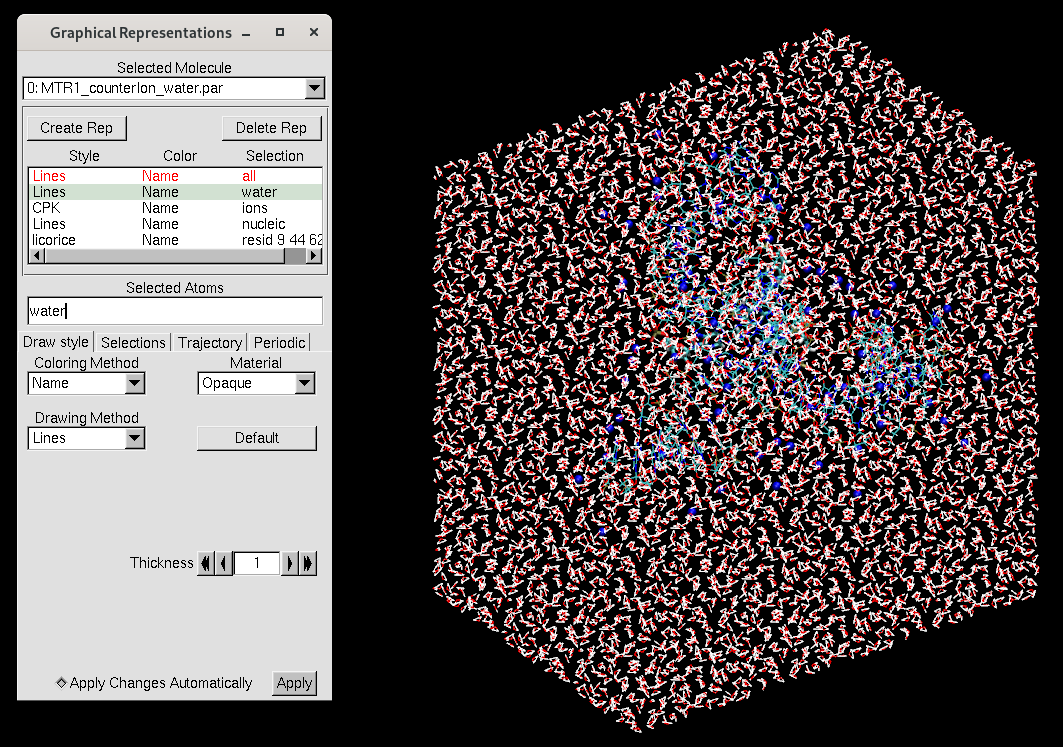
Figure 7. VMD representation of the MTR1 ribozyme in an octahedral solvation box.
The representations now seperate the water and ions rather than referring to just solvent. Here are the contents of MTR_waterreps.txt:
# MTR1 solvated representations

display depthcue off

mol showrep top 0 off

# water
mol selection {water}
mol representation Lines
mol addrep top

# Ions (vmd thinks the ligand is solvent, so exclude it)
mol selection {ions}
mol representation CPK 2.0
mol addrep top

# RNA
mol selection {nucleic}
mol representation Lines
mol addrep top

# Active site residues
mol selection {resid 9 44 62 69}
mol representation licorice
mol addrep top
3.3.4.4. 3.4 Add bulk ions
Next, bulk Na+ and Cl- ions must be added to the water box in order to reach a target concentration of 0.14 M, corresponding to physiological ionic concentration.
AMBER does not directly compute the number of counterions required to reach a desired bulk ion concentration. Therefore, this number must be calculated explicitly based on the system size, the number of water molecules, and the net charge of the system.
To perform this calculation, we use a helper script provided with the parameterization utilities:
parmutils-GetNumIons.py
This script analyzes an AMBER topology file and reports the number of ions that should be added in order to reach the desired salt concentration.
The content of the script is shown below for reference:
#!/usr/bin/env python3
import sys
import parmed

if len(sys.argv) < 2:
    print("""
GetNumIons.py parm [conc]
    parm    amber parm7 filename (string)
    conc    ion concentration, M (float, optional, default: 0.14)

This script reports:
(1) the number of waters within the parm file
(2) the current counterion (Na/Cl) concentration
(3) the current net charge
(4) the net charge excluding Na/Cl counterions

The script provides the addions tleap-command that should be
used to add enough Na/Cl to neutralize the system and achieve
an excess counterion concentration of 0.14 M, or the
concentration specified by the optional argument.
""")
    exit(0)

WatConc = 55.  # M
IonConc = 0.14 # M
if len(sys.argv) > 2:
    IonConc = float(sys.argv[2])

parm = parmed.load_file(sys.argv[1])
NumWatParm  = 0
Charge  = 0.
NonionCharge = 0.
NaParm = 0
ClParm = 0

for atom in parm:
    Charge += atom.charge
    NonionCharge += atom.charge
    if atom.type == "OW" and atom.residue.name == "WAT":
        NumWatParm += 1
    elif atom.type == "Na+" or atom.type == "K+":
        NaParm += 1
        NonionCharge -= 1
    elif atom.type == "Cl-":
        ClParm += 1
        NonionCharge += 1

ChargeFloat = Charge
NonionChargeFloat = NonionCharge
Charge = int("%.0f" % Charge)
NonionCharge = int("%.0f" % NonionCharge)

Na = ((NumWatParm + NaParm + ClParm) * IonConc / WatConc) \
     - (NonionCharge if NonionCharge < 0 else 0) - NaParm
Cl = ((NumWatParm + NaParm + ClParm) * IonConc / WatConc) \
     + (NonionCharge if NonionCharge > 0 else 0) - ClParm

Na = int("%.0f" % Na)
Cl = int("%.0f" % Cl)

ParmConc = 0.
if NumWatParm > 0:
    ParmConc = min(NaParm, ClParm) * WatConc / (NumWatParm + NaParm + ClParm)

print("Current ion concentration: %.3f M" % ParmConc)
print("Current non-counterion charge: %i %.6f" % (NonionCharge, NonionChargeFloat))
print("Current # WAT:", NumWatParm)
print("Current charge: %i %.6f" % (Charge, ChargeFloat))

if Na < 0 or Cl < 0:
    print("ERROR: You already have too many counterions; don't add more")
    if Na < 0:
        print("ERROR: Remove %i sodium" % (-Na))
    if Cl < 0:
        print("ERROR: Remove %i chlorine" % (-Cl))
else:
    print("tleap cmd: addionsrand mol Na+ %i Cl- %i 6.0" % (Na, Cl))
To obtain the required number of ions, the script must be executed on the AMBER topology file of the solvated system. For example:
python3 parmutils-GetNumIons.py MTR1_counterIon_water.parm7
The output of the script includes the recommended tleap command. In this
case, the following line is produced:
tleap cmd: addionsrand mol Na+ 41 Cl- 41 6.0
This indicates that 41 Na+ and 41 Cl- ions must be added to
the system to reach a bulk salt concentration of
0.14 M – on top of the neutralizing part addions mol NA 0 – with a minimum ion–ion separation of 6 Å.
Inclusion of this line completes everything we wanted to do to build our box. Contents of our stand-alone input file are:
set default nocenter on # Do not recenter the molecule

### Sourcing amber forcefields ###############################################

source leaprc.RNA.OL3 # Sourcing RNA force field OL3 to describe RNA.
source leaprc.water.tip4pew # Sourcing water model TIP4P-Ew
                            # and parameters for corresponding monovalent ions
loadamberparams frcmod.ions234lm_1264_tip4pew # divalent metal ion parameters

### Including non-standard residue parameters ################################

# Ligand O6 methylated guanine
loadoff GUN.lib
loadamberparams GUN.frcmod

# N3 protonated cytosine
loadoff OKC.lib
loadamberparams ./modXNA/dat/frcmod.modxna

### Loading structure from file ##############################################
mol= loadpdb "7v9e_C5.pdb"

### Adding counter ions ######################################################
addions mol NA 0 # Add sodium until charge is zero

### Defining box shape & size with chosen water model ########################
solvateoct mol TIP4PEWBOX 9 # solvate with truncated octahedron box 9A out

### Adding bulk ions to ensure 0.14 M concentration ##########################
addionsrand mol NA 41 CL 41 6.0 # add bulk ions, replacing random waters,
                                # ensuring 6 A distance between ions

### Saving output files  #####################################################
# save parameter and restart files
saveamberparm mol MTR1_counterIon_water_bulk.parm7 MTR1_counterIon_water_bulk.rst7
savepdb mol MTR1_counterIon_water_bulk_amber.pdb
quit
We will use this final input file to build our simulation box.
Run tleap:
[user@cluster] tleap -sf MTR1_counterIon_water_bulk.in
This will generate MTR1_counterIon_water_bulk.parm7 and MTR1_counterIon_water_bulk.rst7 that will be used to perform MD simulations.
MTR1_counterIon_water_bulk.parm7
MTR1_counterIon_water_bulk.rst7
Visually inspect the structure in vmd to get a sense of where ions have been placed.
[user@local] vmd MTR1_counterIon_water_bulk.parm7 MTR1_counterIon_water_bulk.rst7
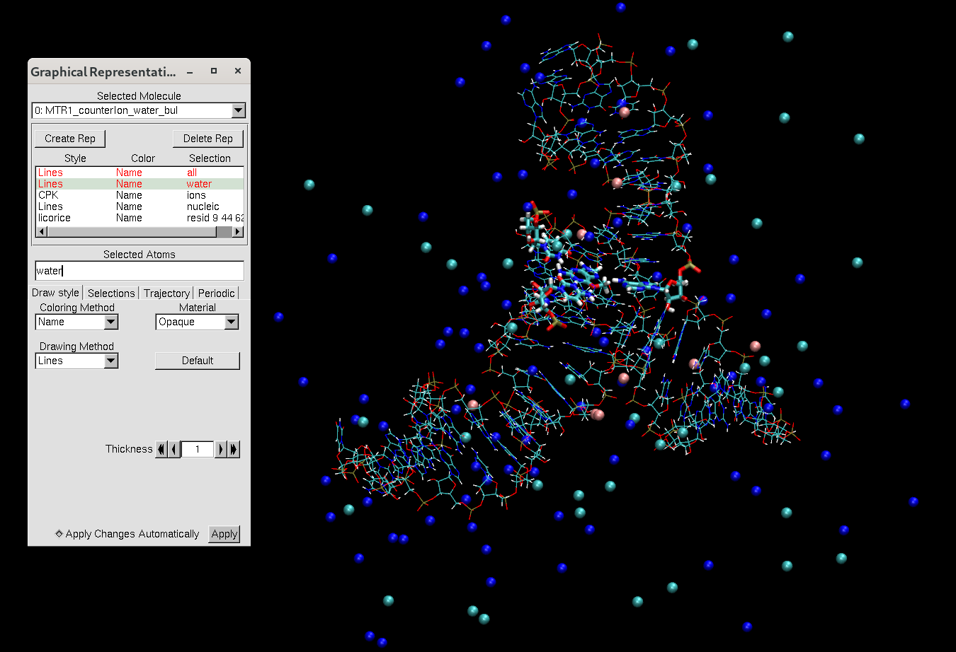
Figure 8. VMD representation of the MTR1 ribozyme with 0.14 M NaCl added to the simulation box.
3.3.5. Divalent metal ion 12-6-4 models with Panteva-Giambasu-York (PGY) pairwise corrections for balanced interactions with nucleic acids
Experimental and theoretical studies have shown that metal ions interact with nucleic acids in two main ways. Electrostatic interactions between the negatively charged nucleic acid backbone and cations lead to a local enrichment of ions around the molecule, known as the ionic atmosphere. In addition to these non-specific interactions, both monovalent and divalent ions can bind more specifically at well-localized sites. In RNA, divalent ions—especially Mg²⁺—can modify local geometry, stabilize tertiary folds, shift the pKa of nearby functional groups, and contribute directly to catalytic activity.
Such binding sites can be identified experimentally using X-ray crystallography, NMR, or spectroscopic techniques. However, these approaches have important limitations: ions are often difficult to identify unambiguously, high and non-physiological ion concentrations are frequently required, and ion positions can be influenced by crystal packing effects. As a result, many questions remain regarding the modes, locations, and strengths of ion binding to nucleic acids, as well as their impact on structure and dynamics. Molecular dynamics simulations therefore provide a valuable complementary approach to study these interactions at the molecular level.
Accurately modeling ion–nucleic acid interactions remains challenging in classical non-polarizable force fields due to the absence of electronic polarization. Fixed atomic charges cannot adapt to the local electrostatic environment, leading to systematic artifacts such as overstabilization of interactions with phosphate groups, underestimation of nucleobase interactions, and an incorrect balance between solvation and direct coordination. As a consequence, divalent ions such as Mg²⁺ may bind too strongly and accumulate unrealistically at the nucleic acid surface.
3.3.5.1. 4.1 How to overcome these limitations?
One option is to use polarizable force fields, which introduce additional terms into the standard functional form to account for electronic polarization explicitly. Approaches based on induced point dipoles and explicit multipoles provide a more realistic physical description of ion–RNA interactions. However, their higher computational cost and the difficulty of parameterization make them challenging to apply routinely, and they are not yet the preferred choice in large-scale biomolecular simulations.
An alternative is to modify the standard potential to incorporate key polarization effects implicitly. Several models follow this strategy by adjusting Lennard–Jones parameters or adding correction terms. The 12-6-4 model extends the classical Lennard–Jones potential by adding a charge-induced dipole interaction term in \(r^{-4}\):
The coefficients \(A_{ij}\) and \(B_{ij}\) correspond to the usual Lennard–Jones parameters, related to \(R_{ij}\) which is the distance at which two particles have a minimum in the LJ potential, while \(\varepsilon_{ij}\) is the well depth :
The additional coefficient \(C_{ij}\) introduces the charge-induced dipole interaction, which is defined as:
where \(\kappa\) is a scaling parameter (in units of Å⁻²) that determines the strength of the \(r^{-4}\) contribution.
However, although the original 12–6–4 model was developed to accurately reproduce bulk hydration properties, it fails to capture experimentally measured affinities for key RNA-binding sites. This limitation motivated the development of the m12–6–4 model, in which only the \(C_{ij}\) coefficients are re-optimized based on experimental data for three representative sites:
non-bridging oxygens of phosphate
N7 of adenine
N7 of guanine
The pairwise coefficient \(C_{ij}\) for an ion interacting with a given atom type is irectly proportional to the polarizability of the atom interacting with the ion \(\alpha\) (in \(\mathrm{Å^3}\)):
This yields several improvements:
more accurate binding free energies between X²⁺-phosphate groups
correct stabilization of nucleobase interactions
an improved balance between solvation and direct coordination
more realistic X²⁺–RNA dissociation kinetics
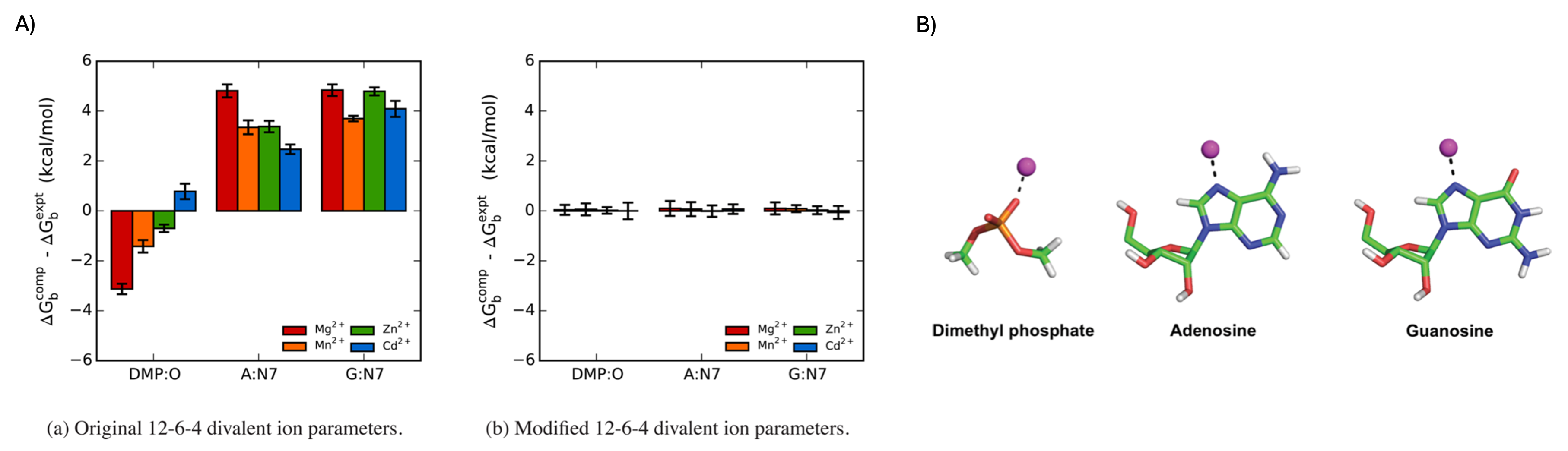
Figure 9. A) Comparison of the errors in the absolute binding free energies for the 12–6–4 (left) and m12–6–4 (right) Mg²⁺, Mn²⁺, Zn²⁺, and Cd²⁺ ion parameters for selected nucleic acid sites. Computed values are averages from three independent simulations, and the error bars correspond to the standard deviations. DMP = dimethyl phosphate, A = adenosine, G = guanosine. B) Model systems and binding sites for which pairwise parameters were tuned to reproduce the reference experimental binding free energies. The magenta sphere represents either Mg²⁺, Mn²⁺, Zn²⁺, or Cd²⁺.
The following files are required to build the 12-6-4 topology and apply the PGY (m12-6-4) pairwise corrections in Amber. These files are already present in the folder on the cluster.
But they can be downloaded directly:
tleap-prep-PDB-2-Amber.intleap input file used to generate the initial Amber topology with the 12-6-4 ion model.1264.shShell script that prepares the ParmEd instruction file and applies the PGY corrections.parmed_1264_na.inParmEd instruction file assigning NAMG/NGMG/OPMG atom types and enabling the PGY corrections.lj_1264_pol.datPolarizability table used by add12_6_4 to compute the \(C_{ij}\) coefficients.
Here, the goal is to learn how to apply these corrections for divalent cations interacting with nucleic acids. We assume you have an AmberTools environment activated.
Nous allons partir des derniers fichiers preparesi: MTR1_counterIon_water_bulk.parm7 MTR1_counterIon_water_bulk.rst7, qui incluent the 12-6-4 Mg²⁺ model. The m12-6-4 (PGY) corrections are applied in a second pass using ParmEd.
3.3.5.2. 4.2 The script 1264.sh
This helper script inserts the proper output file names and runs ParmEd:
#!/bin/bash
# Usage: ./1264.sh SYSTEM

name=$1

cat parmed_1264_na.in > parmed.${name}.in
sed -i '/^outparm/d' parmed.${name}.in

cat <<EOF >> parmed.${name}.in
outparm ${name}_1264.parm7 ${name}_1264.rst7
EOF

parmed -i parmed.${name}.in -p ${name}.parm7 -c ${name}.rst7
Make executable:
chmod +x 1264.sh
3.3.5.3. 4.3 The file parmed_1264_na.in
This file applies the PGY-specific N7(A), N7(G), and OP corrections:
setOverwrite True
change AMBER_ATOM_TYPE :A*,DA*@N7 NAMG
change AMBER_ATOM_TYPE :G*,DG*@N7 NGMG
change AMBER_ATOM_TYPE :*@OP* OPMG

addLJType @%NAMG
addLJType @%NGMG
addLJType @%OPMG

add12_6_4 @%Mg2+ watermodel TIP4PEW polfile lj_1264_pol.dat
printLJMatrix @%Mg2+

outparm NAME.parm7 NAME.rst7
3.3.5.4. 4.4 Polarizabilities (lj_1264_pol.dat)
Below is the full content of the lj_1264_pol.dat file:
H     0.387    Referenced or adopted from Miller JACS,112,8533(1990)
HC    0.387    Referenced or adopted from Miller JACS,112,8533(1990)
H0    0.387    Referenced or adopted from Miller JACS,112,8533(1990)
H1    0.387    Referenced or adopted from Miller JACS,112,8533(1990)
H2    0.387    Referenced or adopted from Miller JACS,112,8533(1990)
H3    0.387    Referenced or adopted from Miller JACS,112,8533(1990)
HA    0.387    Referenced or adopted from Miller JACS,112,8533(1990)
H4    0.387    Referenced or adopted from Miller JACS,112,8533(1990)
H5    0.387    Referenced or adopted from Miller JACS,112,8533(1990)
HO    0.000    Keep its C4 terms consistent with its 12-6 LJ parameters
HS    0.387    Referenced or adopted from Miller JACS,112,8533(1990)
HP    0.387    Referenced or adopted from Miller JACS,112,8533(1990)
HZ    0.387    Referenced or adopted from Miller JACS,112,8533(1990)
h1    0.387    Referenced or adopted from Miller JACS,112,8533(1990)
h2    0.387    Referenced or adopted from Miller JACS,112,8533(1990)
h3    0.387    Referenced or adopted from Miller JACS,112,8533(1990)
h4    0.387    Referenced or adopted from Miller JACS,112,8533(1990)
h5    0.387    Referenced or adopted from Miller JACS,112,8533(1990)
ha    0.387    Referenced or adopted from Miller JACS,112,8533(1990)
hc    0.387    Referenced or adopted from Miller JACS,112,8533(1990)
hn    0.387    Referenced or adopted from Miller JACS,112,8533(1990)
ho    0.000    Keep its C4 terms consistent with its 12-6 LJ parameters
hp    0.387    Referenced or adopted from Miller JACS,112,8533(1990)
hs    0.387    Referenced or adopted from Miller JACS,112,8533(1990)
hx    0.387    Referenced or adopted from Miller JACS,112,8533(1990)
Hc    0.387    Referenced or adopted from Miller JACS,112,8533(1990)
Ha    0.387    Referenced or adopted from Miller JACS,112,8533(1990)
Ho    0.000    Keep its C4 terms consistent with its 12-6 LJ parameters
Hp    0.387    Referenced or adopted from Miller JACS,112,8533(1990)
C     1.352    Referenced or adopted from Miller JACS,112,8533(1990)
C*    1.352    Referenced or adopted from Miller JACS,112,8533(1990)
C4    1.352    Referenced or adopted from Miller JACS,112,8533(1990)
C5    1.352    Referenced or adopted from Miller JACS,112,8533(1990)
CA    1.352    Referenced or adopted from Miller JACS,112,8533(1990)
CB    1.352    Referenced or adopted from Miller JACS,112,8533(1990)
CC    1.352    Referenced or adopted from Miller JACS,112,8533(1990)
CD    1.352    Referenced or adopted from Miller JACS,112,8533(1990)
CK    1.352    Referenced or adopted from Miller JACS,112,8533(1990)
CM    1.352    Referenced or adopted from Miller JACS,112,8533(1990)
CN    1.352    Referenced or adopted from Miller JACS,112,8533(1990)
CO    1.352    Referenced or adopted from Miller JACS,112,8533(1990)
CP    1.352    Referenced or adopted from Miller JACS,112,8533(1990)
CQ    1.352    Referenced or adopted from Miller JACS,112,8533(1990)
CR    1.352    Referenced or adopted from Miller JACS,112,8533(1990)
CS    1.352    Referenced or adopted from Miller JACS,112,8533(1990)
CV    1.352    Referenced or adopted from Miller JACS,112,8533(1990)
CW    1.352    Referenced or adopted from Miller JACS,112,8533(1990)
CY    1.352    Referenced or adopted from Miller JACS,112,8533(1990)
CZ    1.352    Referenced or adopted from Miller JACS,112,8533(1990)
C2    1.352    Referenced or adopted from Miller JACS,112,8533(1990)
C1    1.352    Referenced or adopted from Miller JACS,112,8533(1990)
c     1.352    Referenced or adopted from Miller JACS,112,8533(1990)
c2    1.352    Referenced or adopted from Miller JACS,112,8533(1990)
ca    1.352    Referenced or adopted from Miller JACS,112,8533(1990)
cc    1.352    Referenced or adopted from Miller JACS,112,8533(1990)
cd    1.352    Referenced or adopted from Miller JACS,112,8533(1990)
ce    1.352    Referenced or adopted from Miller JACS,112,8533(1990)
cf    1.352    Referenced or adopted from Miller JACS,112,8533(1990)
cp    1.352    Referenced or adopted from Miller JACS,112,8533(1990)
cq    1.352    Referenced or adopted from Miller JACS,112,8533(1990)
cu    1.352    Referenced or adopted from Miller JACS,112,8533(1990)
cv    1.352    Referenced or adopted from Miller JACS,112,8533(1990)
cx    1.352    Referenced or adopted from Miller JACS,112,8533(1990)
cy    1.352    Referenced or adopted from Miller JACS,112,8533(1990)
cz    1.352    Referenced or adopted from Miller JACS,112,8533(1990)
2C    1.061    Referenced or adopted from Miller JACS,112,8533(1990)
3C    1.061    Referenced or adopted from Miller JACS,112,8533(1990)
C8    1.061    Referenced or adopted from Miller JACS,112,8533(1990)
CI    1.061    Referenced or adopted from Miller JACS,112,8533(1990)
CT    1.061    Referenced or adopted from Miller JACS,112,8533(1990)
CX    1.061    Referenced or adopted from Miller JACS,112,8533(1990)
XC    1.061    Referenced or adopted from Miller JACS,112,8533(1990)
TG    1.061    Referenced or adopted from Miller JACS,112,8533(1990)
c3    1.061    Referenced or adopted from Miller JACS,112,8533(1990)
C7    1.061    Referenced or adopted from Miller JACS,112,8533(1990)
CJ    1.061    Referenced or adopted from Miller JACS,112,8533(1990)
c1    1.283    Referenced or adopted from Miller JACS,112,8533(1990)
cg    1.283    Referenced or adopted from Miller JACS,112,8533(1990)
ch    1.283    Referenced or adopted from Miller JACS,112,8533(1990)
Cg    1.061    Referenced or adoptedfrom Miller JACS,112,8533(1990)
Cy    1.061    Referenced or adopted from Miller JACS,112,8533(1990)
Cp    1.061    Referenced or adopted from Miller JACS,112,8533(1990)
Ck    1.352    Referenced or adopted from Miller JACS,112,8533(1990)
Cj    1.352    Referenced or adopted from Miller JACS,112,8533(1990)
N     1.090    Referenced or adopted from Miller JACS,112,8533(1990)
N*    1.090    Referenced or adopted from Miller JACS,112,8533(1990)
N2    1.090    Referenced or adopted from Miller JACS,112,8533(1990)
N3    1.090    Referenced or adopted from Miller JACS,112,8533(1990)
NA    1.090    Referenced or adopted from Miller JACS,112,8533(1990)
NB    1.090    Referenced or adopted from Miller JACS,112,8533(1990)
NAMG  1.910    From Panteva et al. JPCB, 2015,119,15460
NGMG  1.925    From Panteva et al. JPCB, 2015,119,15460
NAMN  1.770    From Panteva et al. JPCB, 2015,119,15460
NGMN  1.860    From Panteva et al. JPCB, 2015,119,15460
NAZN  1.480    From Panteva et al. JPCB, 2015,119,15460
NGZN  1.640    From Panteva et al. JPCB, 2015,119,15460
NACD  1.580    From Panteva et al. JPCB, 2015,119,15460
NGCD  1.920    From Panteva et al. JPCB, 2015,119,15460
NC    1.090    Referenced or adopted from Miller JACS,112,8533(1990)
ND    1.090    Referenced or adopted from Miller JACS,112,8533(1990)
NL    1.090    Referenced or adopted from Miller JACS,112,8533(1990)
NT    1.090    Referenced or adopted from Miller JACS,112,8533(1990)
NY    1.090    Referenced or adopted from Miller JACS,112,8533(1990)
TN    1.090    Referenced or adopted from Miller JACS,112,8533(1990)
n     1.090    Referenced or adopted from Miller JACS,112,8533(1990)
n1    1.090    Referenced or adopted from Miller JACS,112,8533(1990)
n2    1.090    Referenced or adopted from Miller JACS,112,8533(1990)
n3    1.090    Referenced or adopted from Miller JACS,112,8533(1990)
n4    1.090    Referenced or adopted from Miller JACS,112,8533(1990)
na    1.090    Referenced or adopted from Miller JACS,112,8533(1990)
nb    1.090    Referenced or adopted from Miller JACS,112,8533(1990)
nc    1.090    Referenced or adopted from Miller JACS,112,8533(1990)
nd    1.090    Referenced or adopted from Miller JACS,112,8533(1990)
ne    1.090    Referenced or adopted from Miller JACS,112,8533(1990)
nf    1.090    Referenced or adopted from Miller JACS,112,8533(1990)
nh    1.090    Referenced or adopted from Miller JACS,112,8533(1990)
no    1.090    Referenced or adopted from Miller JACS,112,8533(1990)
Ng    1.090    Referenced or adopted from Miller JACS,112,8533(1990)
O     0.569    Referenced or adopted from Miller JACS,112,8533(1990)
O2    0.569    Referenced or adopted from Miller JACS,112,8533(1990)
O3    0.569    Referenced or adopted from Miller JACS,112,8533(1990)
OD    0.569    Referenced or adoptedfrom Miller JACS,112,8533(1990)
OP    0.569    Referenced or adopted from Miller JACS,112,8533(1990)
OPMG  0.170    From Panteva et al. JPCB, 2015,119,15460
OPMN  0.370    From Panteva et al. JPCB, 2015,119,15460
OPZN  0.510    From Panteva et al. JPCB, 2015,119,15460
OPCD  0.680    From Panteva et al. JPCB, 2015,119,15460
OA    0.637    Referenced or adoptedfrom Miller JACS,112,8533(1990)
OH    0.637    Referenced or adoptedfrom Miller JACS,112,8533(1990)
OS    0.637    Referenced or adoptedfrom Miller JACS,112,8533(1990)
OY    0.637    Added by AG
OZ    0.637    Added by AG
OX    0.637    Added by AG
OW    1.444    From "The Structure and Properties of Water" by Eisenberg & Kauzmann
o     0.569    Referenced or adoptedfrom Miller JACS,112,8533(1990)
oh    0.637    Referenced or adoptedfrom Miller JACS,112,8533(1990)
os    0.637    Referenced or adoptedfrom Miller JACS,112,8533(1990)
ow    1.444    From "The Structure and Properties of Water" by Eisenberg & Kauzmann
Oh    0.637    Referenced or adoptedfrom Miller JACS,112,8533(1990)
Os    0.637    Referenced or adoptedfrom Miller JACS,112,8533(1990)
Oy    0.637    Referenced or adoptedfrom Miller JACS,112,8533(1990)
S     3.000    Referenced or adoptedfrom Miller JACS,112,8533(1990)
SH    3.000    Referenced or adoptedfrom Miller JACS,112,8533(1990)
s     3.000    Referenced or adoptedfrom Miller JACS,112,8533(1990)
s2    3.000    Referenced or adoptedfrom Miller JACS,112,8533(1990)
s4    3.000    Referenced or adoptedfrom Miller JACS,112,8533(1990)
s6    3.000    Referenced or adoptedfrom Miller JACS,112,8533(1990)
sh    3.000    Referenced or adoptedfrom Miller JACS,112,8533(1990)
ss    3.000    Referenced or adoptedfrom Miller JACS,112,8533(1990)
sx    3.000    Referenced or adoptedfrom Miller JACS,112,8533(1990)
sy    3.000    Referenced or adoptedfrom Miller JACS,112,8533(1990)
Sm    3.000    Referenced or adoptedfrom Miller JACS,112,8533(1990)
P     1.538    Referenced or adoptedfrom Miller JACS,112,8533(1990)
p2    1.538    Referenced or adoptedfrom Miller JACS,112,8533(1990)
p3    1.538    Referenced or adoptedfrom Miller JACS,112,8533(1990)
p4    1.538    Referenced or adoptedfrom Miller JACS,112,8533(1990)
p5    1.538    Referenced or adoptedfrom Miller JACS,112,8533(1990)
pb    1.538    Referenced or adoptedfrom Miller JACS,112,8533(1990)
pc    1.538    Referenced or adoptedfrom Miller JACS,112,8533(1990)
pd    1.538    Referenced or adoptedfrom Miller JACS,112,8533(1990)
pe    1.538    Referenced or adoptedfrom Miller JACS,112,8533(1990)
pf    1.538    Referenced or adoptedfrom Miller JACS,112,8533(1990)
px    1.538    Referenced or adoptedfrom Miller JACS,112,8533(1990)
py    1.538    Referenced or adoptedfrom Miller JACS,112,8533(1990)
PX    1.538    Added by AG
F     0.32     From Applequist et al. JACS,94,2952(1972)
Cl    1.91     From Applequist et al. JACS,94,2952(1972)
Br    2.88     From Applequist et al. JACS,94,2952(1972)
I     4.69     From Applequist et al. JACS,94,2952(1972)
f     0.32     From Applequist et al. JACS,94,2952(1972)
cl    1.91     From Applequist et al. JACS,94,2952(1972)
br    2.88     From Applequist et al. JACS,94,2952(1972)
i     4.69     From Applequist et al. JACS,94,2952(1972)
Li    0.029    From Sangster & Atwood J. Phys. C 11,1541(1978)
Li+   0.029    From Sangster & Atwood J. Phys. C 11,1541(1978)
IP    0.2495   From Sangster & Atwood J. Phys. C 11,1541(1978)
Na    0.2495   From Sangster & Atwood J. Phys. C 11,1541(1978)
Na+   0.2495   From Sangster & Atwood J. Phys. C 11,1541(1978)
K     1.0571   From Sangster & Atwood J. Phys. C 11,1541(1978)
K+    1.0571   From Sangster & Atwood J. Phys. C 11,1541(1978)
Rb    1.5600   From Sangster & Atwood J. Phys. C 11,1541(1978)
Rb+   1.5600   From Sangster & Atwood J. Phys. C 11,1541(1978)
Cs    2.5880   From Sangster & Atwood J. Phys. C 11,1541(1978)
Cs+   2.5880   From Sangster & Atwood J. Phys. C 11,1541(1978)
F-    0.9743   From Sangster & Atwood J. Phys. C 11,1541(1978)
Cl-   3.2350   From Sangster & Atwood J. Phys. C 11,1541(1978)
IM    3.2350   From Sangster & Atwood J. Phys. C 11,1541(1978)
Br-   4.5330   From Sangster & Atwood J. Phys. C 11,1541(1978)
I-    6.7629   From Sangster & Atwood J. Phys. C 11,1541(1978)
Be2+  0.0067   Calculated from B3LYP/6-311++G(2d,2p)
Cu2+  0.413    Calculated from B3LYP/6-311++G(2d,2p)
CU    0.413    Calculated from B3LYP/6-311++G(2d,2p)
Ni2+  0.395    Calculated from B3LYP/6-311++G(2d,2p)
Zn    0.344    Calculated from B3LYP/6-311++G(2d,2p)
ZN    0.344    Calculated from B3LYP/6-311++G(2d,2p)
Zn2+  0.344    Calculated from B3LYP/6-311++G(2d,2p)
Co2+  0.447    Calculated from B3LYP/6-311++G(2d,2p)
Cr2+  0.623    Calculated from B3LYP/6-311++G(2d,2p)
Fe    0.518    Calculated from B3LYP/6-311++G(2d,2p)
FE    0.518    Calculated from B3LYP/6-311++G(2d,2p)
Fe2+  0.518    Calculated from B3LYP/6-311++G(2d,2p)
Mg    0.048    Calculated from B3LYP/6-311++G(2d,2p)
MG    0.048    Calculated from B3LYP/6-311++G(2d,2p)
Mg2+  0.048    Calculated from B3LYP/6-311++G(2d,2p)
V2+   0.620    Calculated from B3LYP/6-311++G(2d,2p)
Mn2+  0.534    Calculated from B3LYP/6-311++G(2d,2p)
Hg2+  0.707    Calculated from B3LYP/SDD
Cd2+  0.427    Calculated from B3LYP/SDD
Ca2+  0.477    Calculated from B3LYP/6-311++G(2d,2p)
C0    0.477    Calculated from B3LYP/6-311++G(2d,2p)
Sn2+  3.083    Calculated from B3LYP/SDD
Sr2+  0.813    Calculated from B3LYP/SDD
Ba2+  1.496    Calculated from B3LYP/SDD
HW    0.000    Water hydrogen / dummy atom
hw    0.000    Water hydrogen / dummy atom
EP    0.000    Water hydrogen / dummy atom
EPW   0.000    Water hydrogen / dummy atom
EP1   0.000    Water hydrogen / dummy atom
EP2   0.000    Water hydrogen / dummy atom
LP    0.000    Lone pair site
Al3+  0.031    Calculated from B3LYP/6-311++G(2d,2p)
Fe3+  0.297    Calculated from B3LYP/6-311++G(2d,2p)
Cr3+  0.352    Calculated from B3LYP/6-311++G(2d,2p)
Y3+   0.597    Calculated from B3LYP/SDD
La3+  1.141    Calculated from B3LYP/SDD
Pr3+  1.101    Calculated from B3LYP/SDD
Nd3+  1.047    Calculated from B3LYP/SDD
Sm3+  0.927    Calculated from B3LYP/SDD
Eu3+  0.885    Calculated from B3LYP/SDD
Tm3+  0.675    Calculated from B3LYP/SDD
Lu3+  0.629    Calculated from B3LYP/SDD
Zr4+  0.436    Calculated from B3LYP/SDD
U4+   1.044    Calculated from B3LYP/SDD
Th4+  1.141    Calculated from B3LYP/SDD
M0    0.000    Treat as zero
3.3.5.5. 4.5 Output files
Running:
./1264.sh MTR1_counterIon_water_bulk
produces:
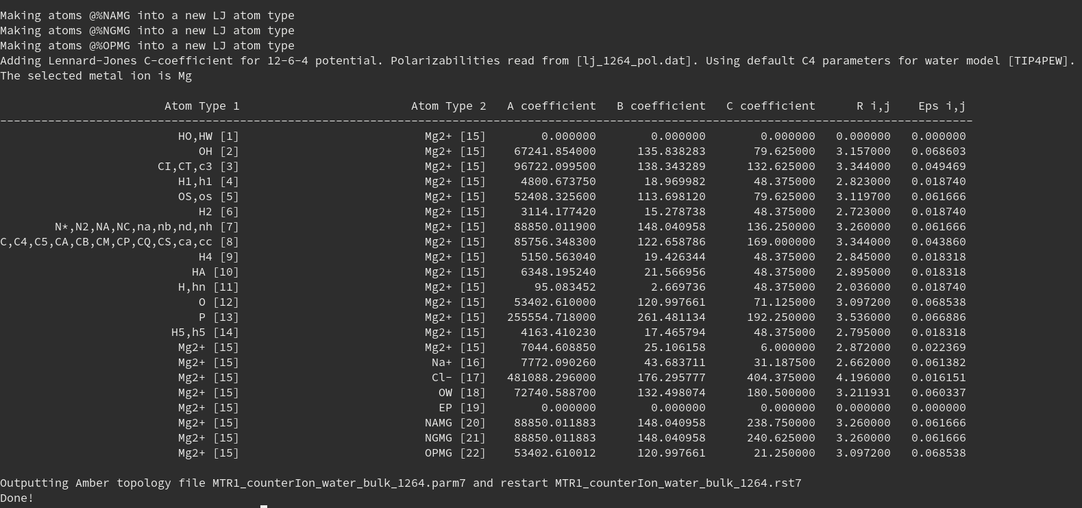
Figure 10. Screenshot of the output showing the interaction matrix involving magnesium.