9. Hands-On Session 9: Principles of Relative Binding Free Energy Calculations
9.1. Learning Objectives
Learn how soft-core potentials are formulated in Amber
Describe the origin of end-point catastrophes, and how smoothstep soft-core potentials help avoid them
Understand the impact of linear, soft-core, and smoothstep soft-core potentials on RBFE calculations.
Learn how to map common-core and soft-core atoms in relative binding free energy calculations.
Understand how different choices of common-core and soft-core atoms can affect the results of relative binding free energy calculations.
9.2. Activities
        flowchart LR

%% ===== inputs =====
A1["Ligand pair<br/>edge in network<br/>two ligands binding same protein"]

%% ===== atom mapping =====
P1{{"<b>[§9.2.2]</b><br/>Map atoms into regions<br/>find_common_core.py"}}
O1["<b>[from §9.2.2.2]</b><br/>Common-core region<br/>shared atoms, not transformed"]
O2["<b>[from §9.2.2.1]</b><br/>Soft-core region<br/>atoms alchemically transformed"]

%% ===== soft-core setup =====
P2{{"<b>[§9.2.1]</b><br/>Set up soft-core potential<br/>smoothstep lambda schedule in Amber"}}
O3["<b>[from §9.2.1.4]</b><br/>Alchemical transformation<br/>lambda-dependent decoupling"]

%% ===== run simulations =====
P3{{"<b>[§9.2.1.4]</b><br/>Run alchemical simulations<br/>across lambda with pmemd.cuda"}}
O4["<b>[from §9.2.1.4]</b><br/>Per-edge free energy<br/>dU/dL sampled per lambda"]

%% ===== network-wide analysis =====
P4{{"<b>[§9.2.3]</b><br/>Combine edges network-wide<br/>edgembar-WriteGraphHtml.py"}}
O5["<b>[from §9.2.3.1]</b><br/>Relative binding free energies<br/>node values, cycle closure errors"]

A1 --> P1
P1 --> O1
P1 --> O2
O1 --> P2
O2 --> P2
P2 --> O3
O3 --> P3
P3 --> O4
O4 --> P4
P4 --> O5

classDef file fill:#fff7e6,stroke:#d98c00,stroke-width:1.5px,color:#111;
classDef program fill:#e8f1ff,stroke:#1f77b4,stroke-width:1.8px,color:#111;
classDef result fill:#eaf7ea,stroke:#2ca02c,stroke-width:1.5px,color:#111;
class A1 file;
class P1,P2,P3,P4 program;
class O1,O2,O3,O4,O5 result;
9.2.1. Introduction to Soft-Core Potentials
In Absolute and Relative Binding Free Energy (RBFE) calculations, one of the key steps is to alchemically disappear a ligand (or transform a ligand into another ligand in the case of RBFE). Thus, to do this, we need to describe how that alchemical transformation will occur, in terms of how the atoms within the TI region’s interactions will be decoupled as a function of lambda. For this purpose, we use soft-core potentials, which are lambda dependent, to ensure that interactions are decoupled smoothly and to avoid singularities during the alchemical transformation.
In the following activity, please download the Jupyter Notebook and follow along.
9.2.1.1. Potential Energies in Amber
Recall, in a molecular simulation the potential energy of the system is described roughly by the following three equations:
Where \(U_{LJ}\) is the Lennard-Jones potential, \(U_{Coul}\) is the Coulomb potential, and \(U_{dir}\) is the direct space part of the Ewald summation for electrostatics. In a soft-core potential, these equations are modified to include lambda dependent terms that ensure smooth decoupling of interactions as lambda goes from 0 to 1.
The core of the problem is that as a ligand is decoupled from the system, the interactions between the ligand and the rest of the system can become singular (i.e. go to infinity) as the ligand’s atoms are turned off.
Note
In this tutorial, we will be considering a radial pair of atoms that are being decoupled, but the same principles apply to fully decoupling a ligand as well (however, this would include more atoms in the soft-core region and require scaling of bonds, angles, and torsions as well).
Let’s first consider the simplest way of decoupling interactions, by simply scaling the interactions by lambda. In this case, the potential energy of the system would be described by the following equations:
In Python, this would look like:
# Sigma, Epsilon, and kT are all set to reduced units for simplicity
sigma, epsilon, kT = 1.0, 1.0, 1.0
beta = 1.0/kT

def U_LJ(r):
    return 4*epsilon*((sigma/r)**12-(sigma/r)**6)

def U_linear(r, lam):
    return (1-lam)*U_LJ(r)

print("U_LJ at r=0.3 sigma:", U_LJ(0.3))
print("U_linear at r=0.3 sigma and lambda=0.5:", U_linear(0.3, 0.5))
print("U_linear at r=0.3 sigma and lambda=0.9:", U_linear(0.3, 0.9))
U_LJ at r=0.3 sigma: 7521218.7241857555
U_linear at r=0.3 sigma and lambda=0.5: 3760609.3620928777
U_linear at r=0.3 sigma and lambda=0.9: 752121.8724185753
As you can see, at low values of the separation distance (r) the potential energy explodes to very high values because its high up on the repulsive wall of the Lennard-Jones potential. With a linear scaling of the interactions, as lambda goes to 1, the potential energy will still be very high at low values of r, which can lead to poor convergence and sampling issues in the alchemical transformation.
9.2.1.2. Soft-Core Potentials
To avoid this issue, we use soft-core potentials which modify the equations for the potential energy to include lambda dependent terms that ensure smooth decoupling of interactions. The traditional soft-core potential for the Lennard-Jones interactions replaces the separation distance (r) with a modified separation distance (r’) that includes lambda dependent terms. The equations for the soft-core potential are as follows:
Where n=6 and m=2 were traditionally used in older forms of the soft-core potential that are no longer recommended (see below), and alpha and beta are soft-core parameters that control the shape of the soft-core potential. The potential energy of the system is then calculated using these modified separation distances.
In Python, this would look like:
def rstar_trad(r, lam, alpha=0.5, n=6):
    return (r**n + alpha*lam*sigma**n)**(1.0/n)

print("Modified separation distance at r=0.3 sigma and lambda=0.5:", rstar_trad(0.3, 0.5))
print("Modified separation distance at r=0.3 sigma and lambda=0.9:", rstar_trad(0.3, 0.9))
Modified separation distance at r=0.3 sigma and lambda=0.5: 0.7940857966009571
Modified separation distance at r=0.3 sigma and lambda=0.9: 0.8756272130490854
As you can see, the modified separation distance (r’) is larger than the original separation distance (r) at low values of r and high values of lambda, which helps to avoid the singularity in the potential energy and allows for smoother decoupling of interactions during the alchemical transformation.
9.2.1.3. Smooth-Step Soft-Core Potentials
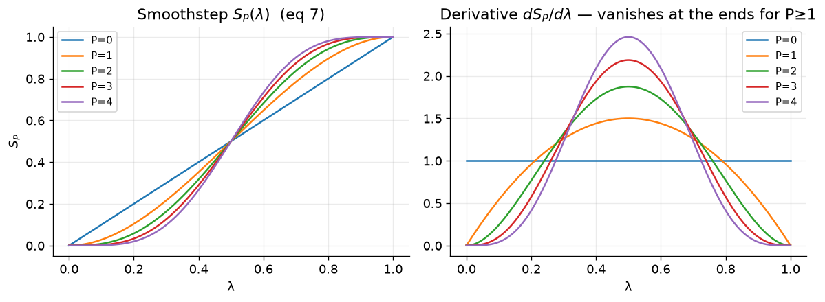
Now, there are some problems with the traditional soft-core potential, such as the fact that \(\alpha\) and \(\beta\) are set independently, which can lead to a mismatch in the decoupling of the Lennard-Jones and Coulomb interactions. Since the short-range repulsive barrier from the Lennard-Jones potential is what keeps particles from collapsing, if that is decoupled faster than the Coulomb interaction it can lead to particle collapse. To address this issue, we use second-order smoothstep functions to ensure that the Lennard-Jones and Coulomb interactions are decoupled in a more consistent manner Tsai et al.[1].
def S(x, P):
    x = np.clip(x, 0, 1)
    return {0: x,
            1: 3*x**2 - 2*x**3,
            2: 6*x**5 - 15*x**4 + 10*x**3,
            3: -20*x**7 + 70*x**6 - 84*x**5 + 35*x**4,
            4: 70*x**9 - 315*x**8 + 540*x**7 - 420*x**6 + 126*x**5}[P]

S2 = lambda x: S(x, 2)


x = np.linspace(0, 1, 400); dx = x[1]-x[0]

fig, ax = plt.subplots(1, 2, figsize=(10, 3.8))

# Make the Left Hand Figure
for P in range(5): ax[0].plot(x, S(x, P), label=f"P={P}")
ax[0].set_title("Smoothstep $S_P(\\lambda)$  (eq 7)"); ax[0].set_xlabel("λ"); ax[0].set_ylabel("$S_P$"); ax[0].legend(fontsize=9)

# Make the Right Hand Figure

for P in range(5): ax[1].plot(x, np.gradient(S(x, P), dx), label=f"P={P}")
ax[1].set_title("Derivative $dS_P/d\\lambda$ — vanishes at the ends for P≥1"); ax[1].set_xlabel("λ"); ax[1].legend(fontsize=9)

fig.tight_layout(); plt.show()
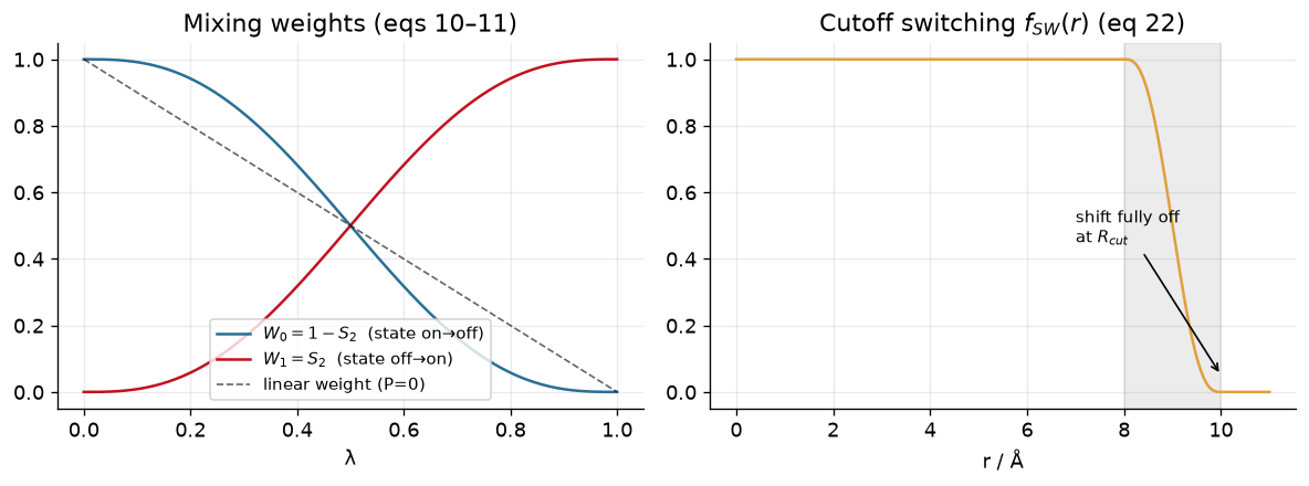
Now, we use these soft-core functions in two ways in an alchemical transformation. The first way is to use the soft-core function as a weight to mix the energy terms of the two end states.
This is defined as follows:
where \(W_0\) and \(W_1\) are the weights for the two end states, and \(S_P(\lambda)\) is the smoothstep function of order P. The potential energy of the system is then calculated as a weighted sum of the potential energies of the two end states, with the weights appearing and leaving with zero derivatives at the endpoints of lambda.
A switching function is also used to recover the true value of r at the nonbonded cutoff, which is defined as follows:
where here, \(R_{cut,i}\) is the distance at which the soft-core potential begins to switch to the true potential, and \(R_{cut,f}\) is the distance at which the soft-core potential fully switches to the true potential. This switching function ensures that the potential energy of the system transitions smoothly from the soft-core potential to the true potential as the separation distance (r) approaches the nonbonded cutoff.
def f_SW(r, Rci, Rcf):
    return 1.0 - S2(np.clip((r - Rci)/(Rcf - Rci), 0, 1))    # eq 22

fig, ax = plt.subplots(1, 2, figsize=(10, 3.8))

ax[0].plot(x, 1-S2(x), color=C["new"], label="$W_0=1-S_2$  (state on→off)")
ax[0].plot(x, S2(x),   color=C["lin"], label="$W_1=S_2$  (state off→on)")
ax[0].plot(x, 1-x, "k--", lw=1, alpha=.6, label="linear weight (P=0)")
ax[0].set_title("Mixing weights (eqs 10–11)"); ax[0].set_xlabel("λ"); ax[0].legend(fontsize=9)

rr = np.linspace(0, 11, 400); Rci, Rcf = 8.0, 10.0

ax[1].plot(rr, f_SW(rr, Rci, Rcf), color=C["trad"]); ax[1].axvspan(Rci, Rcf, color="grey", alpha=.15)
ax[1].set_title("Cutoff switching $f_{SW}(r)$ (eq 22)"); ax[1].set_xlabel("r / Å")
ax[1].annotate("shift fully off\nat $R_{cut}$", (10, 0.05), (7.0, 0.45), fontsize=9, arrowprops=dict(arrowstyle="->"))

fig.tight_layout(); plt.show()
These smoothstep soft-core potentials are then used to generate a new set of modified distances.
We can define these in python as:
def rstar_new(r, lam, alpha=0.5, n=2, switch=False, Rci=8.0, Rcf=10.0):
    fsw = f_SW(r, Rci, Rcf) if switch else 1.0
    return (r**n + alpha*(sigma**n)*S2(lam)*fsw)**(1.0/n)

print("Modified separation distance at r=0.3 sigma and lambda=0.5:", rstar_new(0.3, 0.5))
print("Modified separation distance at r=0.3 sigma and lambda=0.9:", rstar_new(0.3, 0.9))
Modified separation distance at r=0.3 sigma and lambda=0.5: 0.58309518948453
Modified separation distance at r=0.3 sigma and lambda=0.9: 0.7653234610280811
So now, let’s compare what the potential energy looks like for a linear scaling of the interactions, the traditional soft-core potential, and the new smoothstep soft-core potential.
# coupled potentials for a disappearing LJ particle

def U_trad(r, lam, alpha=0.5):                                # eqs 18 + 23, linear weight
    return (1.0 - lam)*U_LJ(rstar_trad(r, lam, alpha))

def U_new(r, lam, alpha=0.5):                                 # eqs 20 + 23, smoothstep weight
    return (1.0 - S2(lam))*U_LJ(rstar_new(r, lam, alpha))

# Plot: the infinite wall at r->0 becomes a finite hill as the particle vanishes
r = np.linspace(0.001, 2.2, 2000)

fig, ax = plt.subplots(1, 3, figsize=(10, 4.0))

for lam in [0.0, 0.4, 0.7, 0.95]:
    ax[0].plot(r, U_linear(r, lam), label=f"λ={lam}")
    ax[1].plot(r, U_trad(r, lam), label=f"λ={lam}")
    ax[2].plot(r, U_new(r, lam),  label=f"λ={lam}")

for a, t in zip(ax, ["Linear", "Traditional Soft-Core", "Smooth-Step Soft-Core)"]):
    a.set_ylim(-1.5, 8); a.set_xlim(0, 2.2); a.set_title(t, fontsize=10.5)
    a.set_xlabel(r"r / $\sigma$"); a.axhline(0, color="k", lw=.6, alpha=.5); a.legend(fontsize=9)

ax[0].set_ylabel(r"U(r; λ) / $\epsilon$")

fig.suptitle("A disappearing particle (λ: 0→1): the hard wall at r→0 becomes finite", fontsize=11)
fig.tight_layout(); plt.show()
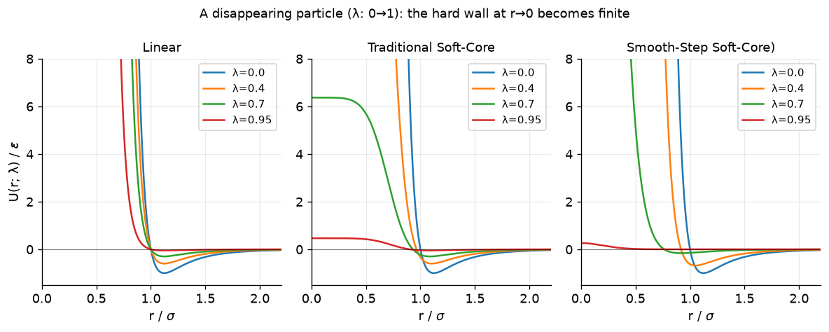
In the above plots, we compare the three scaling approaches. Clearly, in the linear scheme as small separation distances the value of the potential still explodes. The traditional soft-core and smooth-step approaches solve the explosion problem. So why the smoothstep?
Let’s consider what happens in an alchemical transformation. For our 1-D radial pair model, the TI average at a fixed \(\lambda\) is a Boltzmann-weighted integral over the separation (with a 3D volume element \(g(r)=4\pi r^2\)).
We can examine this integral for the three cases.
def moments(Ufun, lam, r_min=0.02, R_box=2.5, N=400000, h=1e-5):

    # Return <DU/DL> and Var(DU/DL) for the 1-D radial pair model at fixed lambda.
    r = np.linspace(r_min, R_box, N)
    g = 4*np.pi*r**2
    w = g*np.exp(-beta*Ufun(r, lam))                 # Boltzmann weight x volume element
    Z = np.trapz(w, r)
    lo, hi = max(lam-h, 0.0), min(lam+h, 1.0)
    dUdl = (Ufun(r, hi) - Ufun(r, lo))/(hi - lo)     # central finite difference
    m1 = np.trapz(w*dUdl, r)/Z
    m2 = np.trapz(w*dUdl*dUdl, r)/Z
    return m1, m2 - m1*m1

lams = np.linspace(0, 0.985, 40)

I = {nm: np.array([moments(f, l) for l in lams])
     for nm, f in [("lin", U_linear), ("trad", U_trad), ("new", U_new)]}

fig, ax = plt.subplots(figsize=(7, 4.2))
ax.plot(lams, I["lin"][:,0],  color=C["lin"],  lw=2, label="linear (no soft-core)")
ax.plot(lams, I["trad"][:,0], color=C["trad"], lw=2, label="traditional soft-core")
ax.plot(lams, I["new"][:,0],  color=C["new"],  lw=2, label="new smoothstep soft-core")
ax.axhline(0, color="k", lw=.6); ax.set_xlabel("λ")
ax.set_ylabel(r"$\langle \partial U/\partial\lambda\rangle_\lambda$  /  ε")
ax.set_title("TI integrand: linear coupling plunges near λ→1 (end-point catastrophe)")
ax.legend(fontsize=9.5); fig.tight_layout(); plt.show()
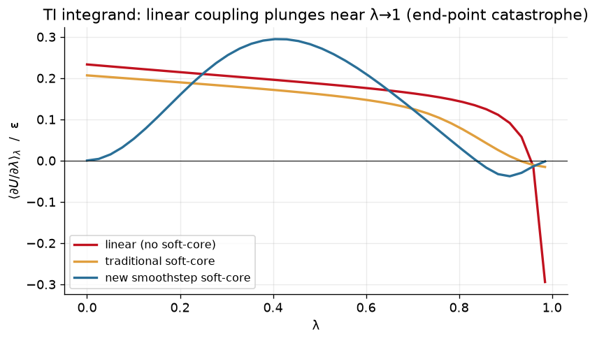
Note the end-point catastrophe that we get with a linear schedule at \(\lambda = 1\). Meanwhile, a traditional soft-core potential performs better (but is still non-zero at the end points). Finally, the new smoothstep soft-core potential approaches both end-points with zero slope.
Note
The recommended values of n and m are n=2 and m=2. Likewise, the suggested values are \(\alpha_{LJ}=0.5\) and \(\alpha_{Coul}=1.0\).
9.2.1.4. Using Soft-Core Potentials in Amber
In the Amber Molecular Dynamics package, we define Soft-Core Potentials through the following parameters:
ifsc=1: Turns on soft-core potentials. These by default reflect the “traditional” soft-core potentials described above.
gti_lam_sch=1: Replaces \(\lambda\) with \(S_P(\lambda)\)
scalpha: Sets the \(\alpha\) term for the soft-core potentials
scbeta: Sets the \(\beta\) term for the soft-core potentials
gti_scale_beta=1: Sets the soft-core potentials to match the functional form described above for the smoothstep soft-core potentials (but doesn’t include smoothing at the non-bonded cutoff). (Also sets scalpha=0.5, scbeta=1.0)
gti_vdw_exp=2: Sets the n parameter for the exponent. (Note - the default is 6).
gti_elec_exp=2: Sets the m parameter for the exponent.
gti_cut_sc=2: Adds the smoothing to the non-bonded cutoff (the \(f_{SW}(r)\) term above)
The lambda schedule is controlled by the file lambda.sch, which looks as follows:
Warning
The Amber Manual currently incorrectly states the defaults for the lambda.sch files. Below are the current actual default values.
TypeGen, smooth_step2, complementary, 0.0, 1.0
TypeBAT, smooth_step2, complementary, 0.0, 1.0
TypeEleRec, smooth_step2, complementary, 0.0, 1.0
TypeEleCC, smooth_step2, complementary, 0.0, 1.0
TypeEleSC, smooth_ step2, complementary, 0.0, 1.0
TypeVDW, smooth_ step2, complementary, 0.0, 1.0
Warning
Your selected parameters for the smoothstep soft-core potentials can significantly impact the stability of your calculations.
Recommended parameter choices are:
gti_vdw_exp=2 gti_elec_exp=2 gti_scale_beta=1 (which sets scalpha=0.5, scbeta=1) and to use the smooth_step2 lambda schedule for the lambda.sch file as shown in the code-block above.
The full comparison of our best-practices compared to defaults is included below.
+------------------+--------+---------------------------+---------------------------+
| Parameter        | Ours   | gti_lam_sch==0            | gti_lam_sch==1            |
+------------------+--------+---------------------------+---------------------------+
| gti_cut_sc       | 2      | 0                         | 0                         |
| gti_ele_exp      | 2      | 2                         | 2                         |
| gti_vdw_exp      | 2      | 6                         | 6                         |
| gti_ele_sc       | 1      | 0                         | 1                         |
| gti_vdw_sc       | 1      | 0                         | 1                         |
| scalpha          | 0.5    | 0.5                       | 0.2                       |
| scbeta           | 1.0    | 12.0                      | 50.0                      |
| gti_auto_alpha   | N/A    | 0                         | 0                         |
+------------------+--------+---------------------------+---------------------------+
You can download an example Amber soft-core input set here: tyk2_softcore.tar.gz
Now let’s try this out. First, download the above tar archive, and then decompress it.
tar -xvf tyk2_softcore.tar.gz
cd tyk2_softcore
In this directory, you will find a parm7 and rst7 file for ejm31, a ligand for Tyk2, in vacuum, along with a sample mdin file (and a script run.sh which runs pmemd.cuda on it).
Let’s start off by running the file. If you look at the parameters above, you can see that we’ve put in place the second-order smoothstep soft-core potential for you to try. Note that clambda=1.0 in this example so that we can see the difference the parameters make.
When you run it, take a look at DU/DL in the produced mdout. You’ll see DU/DL is zero - which is what we expect from the above tutorial.
Let’s switch it up, however. What if we change the settings a bit and revert to traditional soft-core potentials?
cp sp_lam_1.0.mdin ts_lam_1.0.mdin
Edit this file so that the section following clambda looks as follows.
ifsc = 1,
timask1 = ':LIG',
scmask1 = ':LIG',
timask2 = '',
scmask2 = '',
scalpha = 0.5,
scbeta = 1.0,
gti_add_sc = 25,
gti_scale_beta = 0,
gti_lam_sch = 0,
What happened to dU/dL at the endpoint? Note that the DU/DL is no longer zero at the end-point. This is not ideal!
Finally, let’s fully revert to linear scaling.
ifsc = 0,
timask1 = ':LIG',
timask2 = ':LIG',
gti_scale_beta = 0,
gti_lam_sch = 0,
This again gives a DU/DL value that is significantly different from 0.
Take some time to modify parameters (for instance the soft-core parameters in the original smoothstep mdin) to get a feel for how they modulate the behavior. What breaks behavior at the end-point? Also, take some time to look at the entries for the soft-core region in the mdout.
Note
In this final example, gti_add_sc=25 was used which also scales torsions and angles (further scope than the rest of this activity). For more information, please refer to the Amber manual.
9.2.2. Introduction to Atom Mapping
9.2.2.1. Soft-Core Regions for RBFE Calculations
In Relative Binding Free Energy calculations, we are interested in calculating the free energy difference between two ligands binding to the same protein (as opposed to an Absolute Binding Free Energy calculation where we disappear a ligand completely). However, to calculate this free energy difference, we need to alchemically transform one ligand into the other. This transformation is done by identifying a common-core region between the two ligands that is not alchemically transformed, and a soft-core region that is alchemically transformed.
Note
The common-core region is a shared set of atoms present in both ligands that are not alchemically transformed during the simulation.
The soft-core region consists of atoms that are alchemically transformed from one ligand to the other during the simulation. These atoms are typically involved in the chemical differences between the two ligands.
The soft-core region is called “soft-core” because its interactions are lambda dependent and use second-order smoothstep functions to avoid singularities during the alchemical transformation. The choice of which atoms to include in the common-core and soft-core regions can significantly impact the convergence and accuracy of the relative binding free energy calculations.
9.2.2.2. Mapping Soft-Core and Common-Core Atoms
Before we show any code, let’s first consider some example transformations and how we might choose to map the common-core and soft-core atoms. In this tutorial, we will use an example atom mapping script.
Download the following script to your local machine.
#!/usr/bin/env python3
"""Draw two ligands with RDKit and highlight common-core vs soft-core atoms.

This script is aimed at RBFE tutorials where two ligands are compared as an
alchemical pair. It:

1. loads two ligands from either MOL2 files or SMILES strings
2. finds a maximum common substructure (MCS)
3. identifies each ligand's common-core and soft-core atoms
4. writes ChemDraw-style PNG depictions with those regions highlighted

Example
-------
python rdkit_core_softcore_draw.py \
    ejm31/binder_ejm31.mol2 \
    ejm42/binder_ejm42.mol2 \
    --outdir tutorial_drawings

python rdkit_core_softcore_draw.py \
    "CC(=O)Nc1ccc(Oc2ncccn2)cc1" \
    "CC(=O)Nc1ccc(Oc2ncc(C)cn2)cc1" \
    --name-a ligA \
    --name-b ligB
"""

from __future__ import annotations

import argparse
from pathlib import Path

from rdkit import Chem
from rdkit.Chem import AllChem
from rdkit.Chem import Draw
from rdkit.Chem import rdFMCS
from rdkit.Chem import rdDepictor
from rdkit.Chem.Draw import rdMolDraw2D
from rdk_amber import element_from_amber_type, load_amber_mol2


COMMON_CORE_COLOR = (0.55, 0.83, 0.55)
SOFT_CORE_COLOR = (0.95, 0.52, 0.52)


def parse_args() -> argparse.Namespace:
    parser = argparse.ArgumentParser(
        description="Create 2D RDKit drawings with common-core and soft-core highlighting."
    )
    parser.add_argument(
        "ligand_a",
        help="First ligand input: MOL2 file path or SMILES string",
    )
    parser.add_argument(
        "ligand_b",
        help="Second ligand input: MOL2 file path or SMILES string",
    )
    parser.add_argument(
        "--name-a",
        help="Optional display name for ligand A, mainly useful for SMILES input",
    )
    parser.add_argument(
        "--name-b",
        help="Optional display name for ligand B, mainly useful for SMILES input",
    )
    parser.add_argument(
        "--outdir",
        type=Path,
        default=Path("mcss_e2_drawings"),
        help="Output directory for SVG and summary files",
    )
    parser.add_argument(
        "--ignore-hydrogens",
        action="store_true",
        help="Exclude hydrogens from the MCS search and drawings",
    )
    parser.add_argument("--width", type=int, default=500, help="PNG width in pixels")
    parser.add_argument("--height", type=int, default=400, help="PNG height in pixels")
    return parser.parse_args()


def mol2_has_amber_atom_types(path: Path) -> bool:
    in_atom_section = False
    for line in path.read_text(encoding="utf-8").splitlines():
        stripped = line.strip()
        if stripped.startswith("@<TRIPOS>ATOM"):
            in_atom_section = True
            continue
        if stripped.startswith("@<TRIPOS>") and in_atom_section:
            break
        if not in_atom_section or not stripped or stripped.startswith("#"):
            continue

        fields = stripped.split()
        if len(fields) < 6:
            continue

        atom_type = fields[5]
        if "." in atom_type:
            continue
        if element_from_amber_type(atom_type) is not None:
            return True

    return False


def ligand_name(path: Path) -> str:
    stem = path.stem
    if stem.startswith("binder_"):
        return stem.removeprefix("binder_")
    return stem


def sanitize_name(name: str) -> str:
    sanitized = "".join(ch if ch.isalnum() or ch in {"-", "_"} else "_" for ch in name)
    sanitized = sanitized.strip("_")
    return sanitized or "ligand"


def infer_ligand_name(raw_input: str, explicit_name: str | None) -> str:
    if explicit_name:
        return explicit_name

    path = Path(raw_input)
    if path.exists():
        return ligand_name(path)

    return sanitize_name(raw_input[:24])


def load_mol_from_path(path: Path, keep_hydrogens: bool) -> Chem.Mol:
    if mol2_has_amber_atom_types(path):
        mol = load_amber_mol2(str(path), remove_hs=not keep_hydrogens)
    else:
        mol = Chem.MolFromMol2File(str(path), removeHs=not keep_hydrogens)
    if mol is None:
        raise ValueError(f"Failed to read MOL2 file: {path}")
    return mol


def load_smiles(smiles: str, keep_hydrogens: bool) -> Chem.Mol:
    mol = Chem.MolFromSmiles(smiles)
    if mol is None:
        raise ValueError(f"Failed to parse SMILES string: {smiles}")

    if keep_hydrogens:
        mol = Chem.AddHs(mol)

    return mol


def load_ligand(raw_input: str, keep_hydrogens: bool, name: str | None) -> tuple[Chem.Mol, str]:
    path = Path(raw_input)
    ligand_label = infer_ligand_name(raw_input, name)
    if path.exists():
        mol = load_mol_from_path(path, keep_hydrogens)
    else:
        mol = load_smiles(raw_input, keep_hydrogens)

    mol.SetProp("_Name", ligand_label)
    return mol, ligand_label


def find_common_core(mol_a: Chem.Mol, mol_b: Chem.Mol) -> tuple[list[int], list[int], Chem.Mol]:
    mcs = rdFMCS.FindMCS(
        [mol_a, mol_b],
        atomCompare=rdFMCS.AtomCompare.CompareElements,
        bondCompare=rdFMCS.BondCompare.CompareOrderExact,
        ringMatchesRingOnly=True,
        completeRingsOnly=True,
        maximizeBonds=True,
        timeout=30,
    )
    if mcs.canceled or not mcs.smartsString:
        raise RuntimeError("MCS search failed or timed out without a result.")

    query = Chem.MolFromSmarts(mcs.smartsString)
    if query is None:
        raise RuntimeError("RDKit returned an invalid SMARTS for the common core.")

    match_a = list(mol_a.GetSubstructMatch(query))
    match_b = list(mol_b.GetSubstructMatch(query))
    if not match_a or not match_b:
        raise RuntimeError("Could not map the common-core SMARTS back onto both ligands.")

    return match_a, match_b, query


def orient_molecules_on_common_core(mol_a: Chem.Mol, mol_b: Chem.Mol, query: Chem.Mol) -> None:
    """Generate matched 2D depictions so the common core keeps one orientation."""
    # Use a sanitized ligand as the 2D reference.
    # The raw MCS SMARTS query can match substructures, but it may not have ring
    # information initialized, which causes depiction matching to fail for
    # fused-ring systems in newer RDKit builds.
    rdDepictor.Compute2DCoords(mol_a)
    rdDepictor.StraightenDepiction(mol_a, minimizeRotation=True)

    AllChem.GenerateDepictionMatching2DStructure(
        mol_b,
        mol_a,
        refPatt=query,
        acceptFailure=False,
    )


def atom_labels(mol: Chem.Mol, atom_indices: list[int]) -> list[str]:
    labels = []
    for atom_idx in atom_indices:
        atom = mol.GetAtomWithIdx(atom_idx)
        pdb_name = atom.GetPDBResidueInfo().GetName().strip() if atom.GetPDBResidueInfo() else ""
        label = pdb_name or f"{atom.GetSymbol()}{atom_idx + 1}"
        labels.append(label)
    return labels


def highlight_atom_colors(mol: Chem.Mol, common_core_atoms: list[int]) -> tuple[list[int], dict[int, tuple[float, float, float]]]:
    common_core = set(common_core_atoms)
    soft_core = [atom.GetIdx() for atom in mol.GetAtoms() if atom.GetIdx() not in common_core]
    atom_colors = {idx: COMMON_CORE_COLOR for idx in common_core_atoms}
    atom_colors.update({idx: SOFT_CORE_COLOR for idx in soft_core})
    return common_core_atoms + soft_core, atom_colors


def draw_combined_png(
    mol_a: Chem.Mol,
    mol_b: Chem.Mol,
    match_a: list[int],
    match_b: list[int],
    out_path: Path,
    width: int,
    height: int,
) -> None:
    highlight_atoms_a, atom_colors_a = highlight_atom_colors(mol_a, match_a)
    highlight_atoms_b, atom_colors_b = highlight_atom_colors(mol_b, match_b)

    drawer = rdMolDraw2D.MolDraw2DCairo(width * 2, height, width, height)
    opts = drawer.drawOptions()
    opts.useBWAtomPalette()
    opts.bondLineWidth = 2
    opts.fixedBondLength = 32
    opts.padding = 0.08
    opts.legendFontSize = 18
    opts.atomHighlightsAreCircles = False
    opts.fillHighlights = True

    prepared_mols = [Draw.PrepareMolForDrawing(mol_a), Draw.PrepareMolForDrawing(mol_b)]
    drawer.DrawMolecules(
        prepared_mols,
        legends=[mol_a.GetProp("_Name"), mol_b.GetProp("_Name")],
        highlightAtoms=[highlight_atoms_a, highlight_atoms_b],
        highlightAtomColors=[atom_colors_a, atom_colors_b],
        highlightBonds=[[], []],
    )
    drawer.FinishDrawing()
    out_path.write_bytes(drawer.GetDrawingText())


def write_summary(
    path: Path,
    mol_a: Chem.Mol,
    mol_b: Chem.Mol,
    match_a: list[int],
    match_b: list[int],
    query: Chem.Mol,
) -> None:
    core_a = atom_labels(mol_a, match_a)
    core_b = atom_labels(mol_b, match_b)
    soft_a = atom_labels(
        mol_a,
        [atom.GetIdx() for atom in mol_a.GetAtoms() if atom.GetIdx() not in set(match_a)],
    )
    soft_b = atom_labels(
        mol_b,
        [atom.GetIdx() for atom in mol_b.GetAtoms() if atom.GetIdx() not in set(match_b)],
    )

    lines = [
        f"{mol_a.GetProp('_Name')}: {mol_a.GetNumAtoms()} atoms",
        f"{mol_b.GetProp('_Name')}: {mol_b.GetNumAtoms()} atoms",
        f"common_core_atoms: {query.GetNumAtoms()}",
        f"{mol_a.GetProp('_Name')}_common_core: {', '.join(core_a) if core_a else 'none'}",
        f"{mol_b.GetProp('_Name')}_common_core: {', '.join(core_b) if core_b else 'none'}",
        f"{mol_a.GetProp('_Name')}_soft_core: {', '.join(soft_a) if soft_a else 'none'}",
        f"{mol_b.GetProp('_Name')}_soft_core: {', '.join(soft_b) if soft_b else 'none'}",
    ]
    path.write_text("\n".join(lines) + "\n", encoding="utf-8")


def main() -> None:
    args = parse_args()
    args.outdir.mkdir(parents=True, exist_ok=True)

    keep_hydrogens = not args.ignore_hydrogens

    mol_a, name_a = load_ligand(args.ligand_a, keep_hydrogens, args.name_a)
    mol_b, name_b = load_ligand(args.ligand_b, keep_hydrogens, args.name_b)

    match_a, match_b, query = find_common_core(mol_a, mol_b)
    orient_molecules_on_common_core(mol_a, mol_b, query)

    png = args.outdir / f"{sanitize_name(name_a)}~{sanitize_name(name_b)}.png"
    summary = args.outdir / "common_core_summary.txt"

    draw_combined_png(mol_a, mol_b, match_a, match_b, png, args.width, args.height)
    write_summary(summary, mol_a, mol_b, match_a, match_b, query)

    print(f"Wrote {png}")
    print(f"Wrote {summary}")


if __name__ == "__main__":
    main()
This script uses the rdk-amber package (a small compatibility library to enable mol2 files with amber atom types to be turned into rdkit molecules.)
To use this package, run this (ideally in a conda/other virtual python environment).
pip install rdk-amber
Once your environment is set up, you can download the following mol2 files in a tar.gz format here:
Try running the script on these mol2 files.
tar -xvf atom_mapping.tar.gz
cd atom_mapping
python find_common_core.py binder_ejm31.mol2 binder_jmc27.mol2
This will write a directory with a png image, open that and you should see something like this.
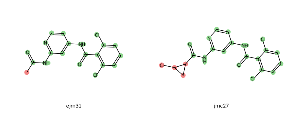
Here, the red highlighted groups are in the soft-core region and the green highlighted groups are in the common-core region.
Try this for the remaining mol2 files - do you notice anything about these soft-core regions?
9.2.2.3. Considerations for Picking Soft-Core Regions
In general, there are a few best practices to use when generating soft-core regions:
There should only be one soft-core region per transformation (e.g. all red regions with the tool above should be contiguous)
Dihedrals only obtain the benefit of enhanced sampling (dihedral parameters turned off) when soft-core regions fully cover the bond.
If the soft-core region gets too large, then this can negatively impact the replica exchange acceptance ratios.
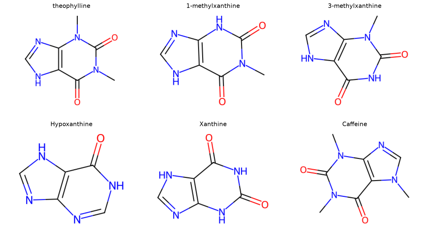
Now let’s look at a few examples that are not from Tyk2. These come from the paper by Ali Rasouli and co-workers Rasouli et al.[2], which looked at a theophylline-binding RNA aptamer.
We will use the same script as before, but with smiles strings. In the paper, they looked at six molecules that were theophylline-like.
import matplotlib.pyplot as plt
from rdkit import Chem
from rdkit.Chem import Draw

smiles_dict = {
    "theophylline": "CN1C2=C(C(=O)N(C1=O)C)NC=N2",
    "1-methylxanthine": "CN1C(=O)NC2=C(NC=N2)C1=O",
    "3-methylxanthine": "CN1C2=C(NC=N2)C(=O)NC1=O",
    "Hypoxanthine": "O=C1NC=Nc2nc[nH]c12",
    "Xanthine": "C1=NC2=C(N1)C(=O)NC(=O)N2",
    "Caffeine": "CN1C=NC2=C1C(=O)N(C(=O)N2C)C",
}

fig, axes = plt.subplots(2, 3, figsize=(12, 7))

for ax, (name, smiles) in zip(axes.flat, smiles_dict.items()):
    mol = Chem.MolFromSmiles(smiles)
    img = Draw.MolToImage(mol, size=(300, 220))
    ax.imshow(img)
    ax.set_title(name, fontsize=12)
    ax.axis("off")

fig.tight_layout()
plt.show()
Now let’s call the find_common_core.py script with the SMILES strings for caffeine and xanthine.
python find_common_core.py "C1=NC2=C(N1)C(=O)NC(=O)N2" "CN1C=NC2=C1C(=O)N(C(=O)N2C)C" --name-a xanthine --name-b caffeine
Here, note the name-a and name-b flags make a more convenient output png filename.
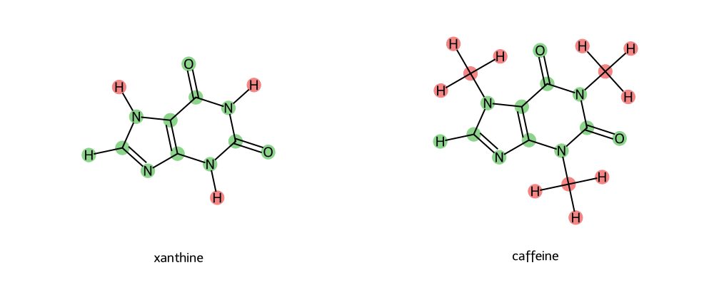
How do these soft-core regions look? Let’s check how they compare to our guidelines above.
Only One Soft-Core Region (FAIL!)
Now - this is a particularly tricky case. You could expand the soft-core region to try to correct this; however, in reality this would essentially engulf the entirety of both molecules. You could try to look for intermediate transformations (however, in this case there is only one valid transformation linking caffeine to a potential network). Can you identify which that is? Try to use the atom-mapping tool to find out. (Answer toggle below)
Caffeine~Theophylline is a valid transformation.
So what would you do?
Three options:
Generate a network, but only connect Caffeine via one edge. Downside: No cycle closure information about caffeine.
Generate a network, but define a pseudo-ligand that bridges the soft-core potential gap. Downside: Can be difficult to generate the molecule, more simulations.
Generate a network, but connect caffeine to other ligands with Counterpoised Binding Free Energy (CBFE) calculations instead. Downside: this is more challenging to resolve and uses a different method.
Note
Counterpoised Binding Free Energies (CBFE)
For cases where it is hard to draw a transformation, or because you want to connect two RBFE networks with differing scaffolds, you can no longer use the RBFE-like infrastructure that we have discussed above. Instead, a more challenging technique is needed: CBFE. Like RBFE, CBFE involves two ligands transforming into one another; however, unlike RBFE, it is a complete transformation without a common core. One ligand is completely disappearing while another ligand is completely appearing. Thus, it is closer to two ABFE calculations run in opposite directions simultaneously. Since both ligands decouple simultaneously, Boresch restraints are often used between the ligands to keep them aligned with one another (as opposed to between the protein and the ligand, as is the case in ABFE).
More information on CBFE can be found in the work by Tsai and co-workers. Tsai et al.[3]
Note
In a later HandsOn Tutorial (Number 13) we will demonstrate how to use AmberStudio to actually set up and run an RBFE calculation on Tyk2; however, for the remainder of this session we will look at an example analysis set for an RBFE network run previously.
9.2.3. Introduction to Network-Wide Analysis
FE-Toolkit provides, for RBFE calculations, the ability to perform network-wide analysis for comparing many different Relative Binding Free Energy (RBFE) calculations in a concerted way.
This is done by calling edgembar-WriteGraphHtml.py from FE-Toolkit on the Python files generated during analysis.
Note
An example call for edgembar-WriteGraphHtml.py is included below, but is out of scope for this tutorial.
Running: edgembar-WriteGraphHtml.py -o analysis/Graph.html $(ls analysis/*~*.py)
9.2.3.1. Examining a Network-Wide Analysis Result
In this activity, you will be working with a set of completed RBFE simulations for Tyk2. These include 16 ligands, with 31 independent simulations forming edges between these ligands.
Open the FE-Toolkit network graph report here: Graph.html
When you first load the HTML file, you will see at the top of the file a map of the RBFE network (in this case three ligands) with a variety of controls.
You can use these controls to customize the display of the results, including the coloring of nodes, and the coloring and thickness of edges based on various metrics.
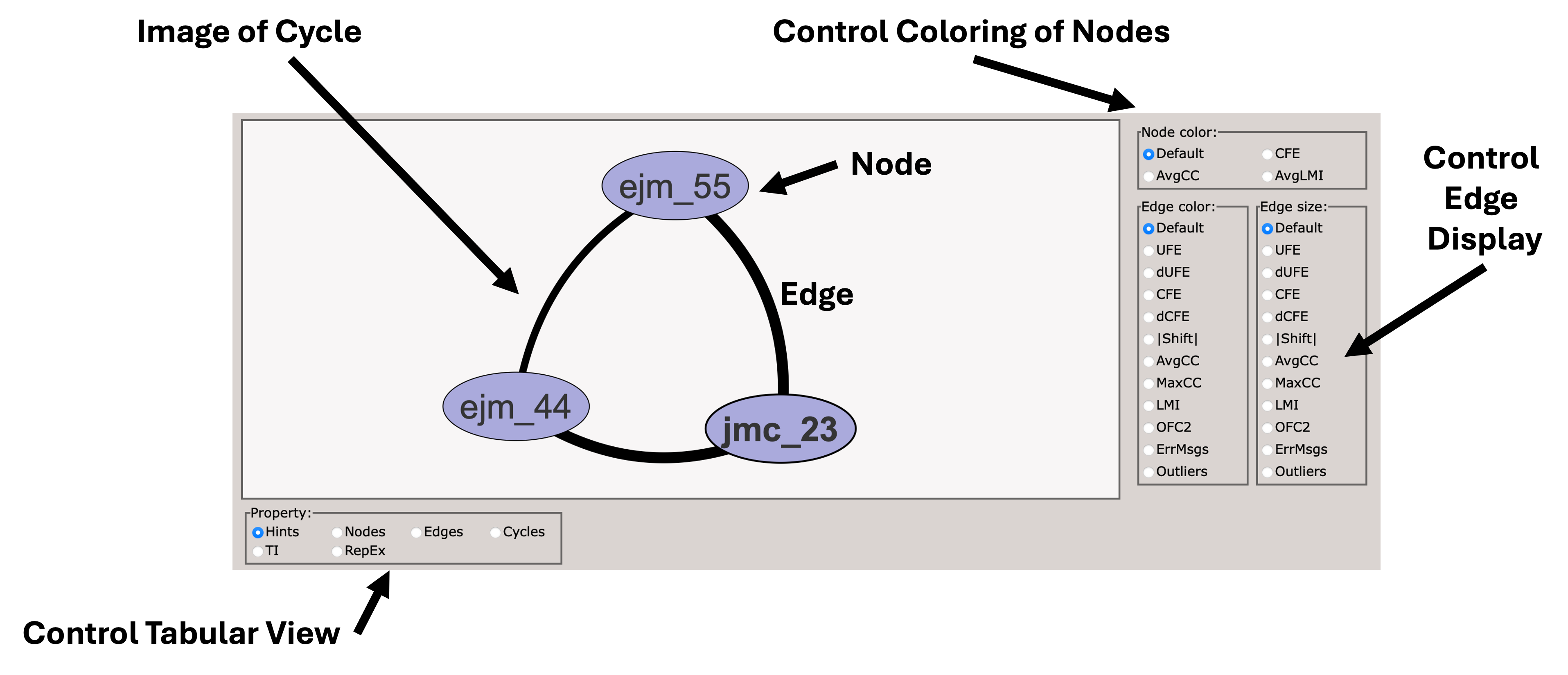
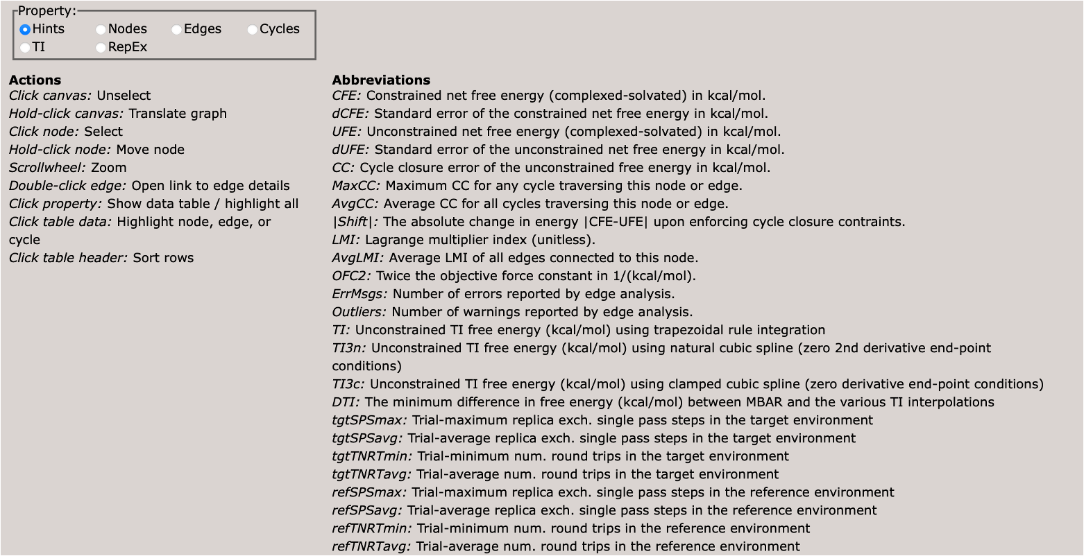
Scrolling down, you will see a control panel that allows you to display a variety of views. The default is a help pane which describes various important abbreviations.
This section describes various important abbreviations used in the graph display.
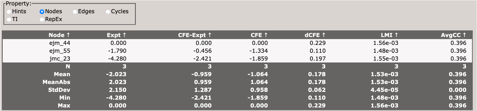
This section describes the free energy of individual nodes (ligands) in the network (relative to an arbitrary reference ligand).
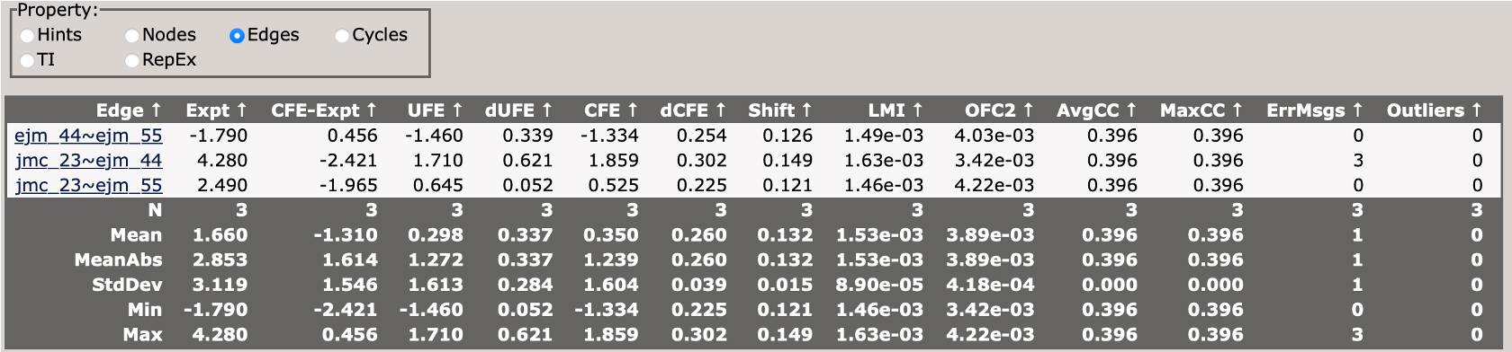
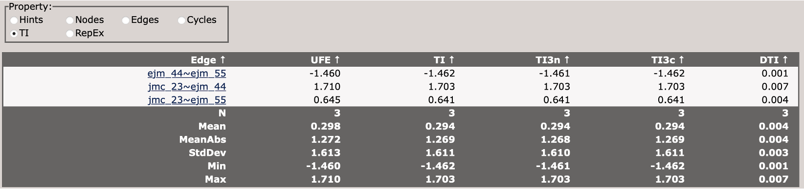
This section describes the free energy differences between pairs of ligands (edges) in the network.
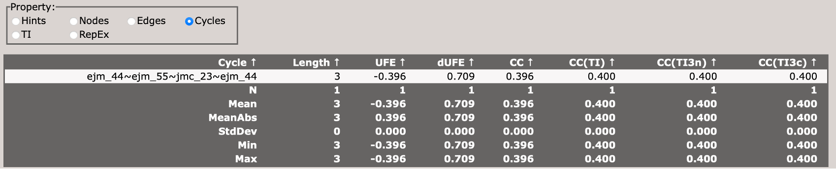
This section describes the cycle closure errors for cycles in the network.
This compares different TI analysis approaches and how well they agree with BAR.
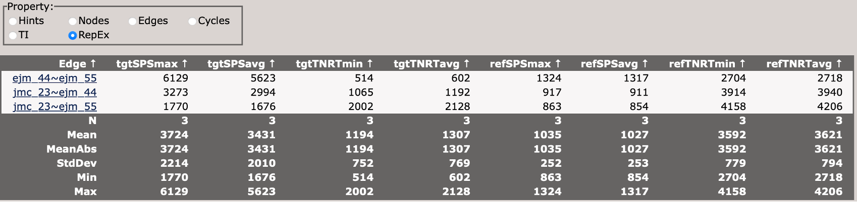
This section describes the replica exchange statistics for each edge in the network.
Now take some time to explore the file, and each tab. Each edge from the network can be accessed from the Edges panel.
With the remainder of your time:
Try to make a plot of the constrained free energy versus experiment. How does the R^2 perform? Is the RMSD reasonable? How close to 1 is the slope?
Color the edges in the main diagram by the maximum cycle closure error. Do any of the ligands stand out to you as problematic? Are there any edges that should be reconsidered and rerun?
Color the edges in the main diagram by ErrMsgs. Open the edge with the worst errors from the Edges panel. Where are those errors coming from? Is it all trials that are having problems, or just one problematic trial?
Look at the cycle closure errors in the Cycles panel. Sort by CC. Which cycle is the worst? Does it include the edge we identified from above?