5. Hands-On Session 5: Perform SASM calculations to study catalytic mechanisms of a ribozyme
5.1. Learning Objectives
Perform QM/MM umbrella sampling simulations with AMBER using semi-empirical QM model
Use NDFES program to set up and analyze simulations
Observe the effects of number of reaction coordinates on the free energy profile
Use SASM to find the minimum free energy path for a reaction in multiple dimensions
Interpret the free energy profile in the context of reaction mechanism
5.2. Relevant literature
5.3. Activities
5.3.1. Workflow
        flowchart LR

%% ===== prepare initial guess =====
A1["Input files<br/>reactant.disang<br/>intermediate.disang<br/>product.disang<br/>img.disang, equil.mdin"]
P1{{"<b>[§5.4]</b><br/>Prepare initial guess path<br/>ndfes-path-prepguess.py"}}
O1["<b>[from §5.4]</b><br/>Window disangs for guess<br/>img01..32.disang"]
A1 --> P1
P1 --> O1

%% ===== run SASM string simulations =====
P2{{"<b>[§5.5]</b><br/>Run SASM string iterations<br/>sander.MPI"}}
O2["<b>[from §5.5]</b><br/>Sampled string data<br/>img01..32.dumpave"]
O1 --> P2
P2 --> O2

%% ===== analyze the set of strings =====
P3{{"<b>[§5.6]</b><br/>Build metafile and FE surface<br/>ndfes-path-analyzesims.py, ndfes_omp"}}
O3["<b>[from §5.6]</b><br/>Combined metafile and chk<br/>metafile.all, metafile.all.chk"]
O2 --> P3
P3 --> O3

P4{{"<b>[§5.6]</b><br/>Optimize path and plot surface<br/>ndfes-path_omp, Example2d.py"}}
O4["<b>[from §5.6.1/.2/.3]</b><br/>MFEP per pathway<br/>path.wavg.0.dat, path png"]
O3 --> P4
P4 --> O4

%% ===== visualize path progression =====
P5{{"<b>[§5.7]</b><br/>Make string progression movie<br/>Make2dMovie.sh, ffmpeg"}}
O5["<b>[from §5.7]</b><br/>Convergence movie<br/>movie.sims.mp4"]
O4 --> P5
P5 --> O5

%% ===== compare DFTB3 vs delta-MLP grid =====
A6["Input files<br/>metafile.string<br/>metafile.chk"]
P6{{"<b>[§5.8]</b><br/>Optimize DFTB3 path on grid<br/>ndfes-path_omp, Example2d.py"}}
O6["<b>[from §5.8]</b><br/>DFTB3 vs delta-MLP PMFs<br/>path.wavg.0.dat, grid path png"]
O4 --> P6
A6 --> P6
P6 --> O6

%% ===== bootstrap error analysis =====
A7["Input files<br/>tr1..tr4 dumpaves<br/>metafile.current"]
P7{{"<b>[§5.9]</b><br/>Bootstrap error analysis<br/>analyze.sh: ndfes_omp, ndfes-AvgFESs.py, ndfes-path_omp"}}
O7["<b>[from §5.9]</b><br/>PMF with error bars<br/>path.avg.wavg.0.dat"]
A7 --> P7
P7 --> O7

classDef file fill:#fff7e6,stroke:#d98c00,stroke-width:1.5px,color:#111;
classDef program fill:#e8f1ff,stroke:#1f77b4,stroke-width:1.8px,color:#111;
classDef result fill:#eaf7ea,stroke:#2ca02c,stroke-width:1.5px,color:#111;
class A1,A6,A7 file;
class P1,P2,P3,P4,P5,P6,P7 program;
class O1,O2,O3,O4,O5,O6,O7 result;
Download the necessary inputs for this activity:
Attention
Copy the directory to your working directory
cp -r /PATH2Files/HandsOn5-String.tar.gz ./
tar -xzvf HandsOn5-String.tar.gz
cd HandsOn5-String
Load the amber module:
{{amberload}}
You will also periodically need to use xmgrace to plot your results. Load the xmgrace module:
{{xmgraceload}}
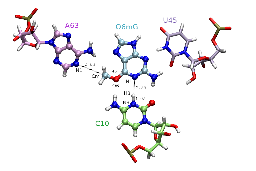
Given that the barrier to methyl transfer was so high, we will now include an additional coordinate for proton transfer. This evaluates the potential impact of general acid catalysis on the mechanism and free energy profile. However, with this new degree of freedom, it is unclear what the minimum free energy path is to get from reactants to products, so we need a method to navigate the multidimensional free energy landscape.
In this section you will analyze data from a series of surface accelerated string method (SASM) simulations that sample the reaction space with two reaction coordinates: RC1 = |RC10:N3-H| - |RmG:N1 - RH| and RC2 = |RO6mG:O6 - RCm| - | RA63:N1 - RCm |. The process of generating the inputs and equilibrating the windows for two dimensions would be analogous to the 1D example, except another reaction coordinate is specified in the img.disang file, and adequate window spacing must be maintained in both dimensions.
The surface accelerated string method is an iterative procedure starting from an initial guess of the path that seeks to convergence upon the minimum free energy path. This method converges rapidly by running a set of umbrella sampling simulations on a given path, and after each iteration optimizing the path on the collective free energy surface from all of the sampling iterations performed up to that point. Every other string iteration, it performs “exploratory” simulations where the umbrella centers are placed just beyond the point on the minimum free energy path to thoroughly sample the vicinity of the path to avoid falling into local minima and create a rigorous free energy surface.
5.4. Preparing an initial guess containing and intermediate
There are 3 simulation directories provided called PT, MT, and linear. These correspond to 3 initial guesses of the path from which the pathfinding was initiated. PT is a stepwise pathway where the proton is transferred followed by the methyl transfer in a perfectly stepwise fashion. MT follows the opposite pathway where the methyl transfer occurs first and the proton transfer occurs second. The linear pathway is a perfectly concerted mechanism where the path is a straight line from reactants to products. At the offset, it is unclear which pathway is most energetically favorable. The activity will use the linear path as the example.
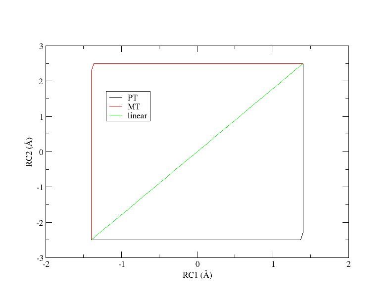
Initial guesses of the minimum free energy path from reactant (lower left corner) to product (upper right corner).
In Hands on session 4, you used ndfes-path-prepguess.py to prepare input files for a 1 dimensional path that linearly interpolated from reactant to products. In this section, we will generate an initial guess where the proton transfer (PT) preceeds the methyl transfer (MT) step, motivated by the 2D grid that we saw in the previous session to demonstrate how one can set up a guess beyond a straight line.
Navigate to the start directory for the PT path:
cd PT/start
ls
intermediate.disang  product.disang  reactant.disang  reactant.rst7
The key is to supply intermediate.disang with the reaction coordinates set to (1.4,-2.5). Therefore we will linearly interpolate from reactant.disang to intermediate.disang, then from intermediate.disang to product.disang. Run NDFES to generate the equil directory:
ndfes-path-prepguess.py -d ../template/img.disang -i ../template/equil.mdin --min reactant.disang --min intermediate.disang --min product.disang --pad 3 -n 32 -o ../equil
cp reactant.rst7 init/init001.rst7
  1    -1.400    -2.500   init/img001.disang
  2    -1.148    -2.500   init/img002.disang
  3    -0.897    -2.500   init/img003.disang
  4    -0.645    -2.500   init/img004.disang
  5    -0.394    -2.500   init/img005.disang
  6    -0.142    -2.500   init/img006.disang
  7     0.110    -2.500   init/img007.disang
  8     0.361    -2.500   init/img008.disang
  9     0.613    -2.500   init/img009.disang
  10     0.865    -2.500   init/img010.disang
  11     1.116    -2.500   init/img011.disang
  12     1.368    -2.500   init/img012.disang
  13     1.400    -2.281   init/img013.disang
  14     1.400    -2.029   init/img014.disang
  15     1.400    -1.777   init/img015.disang
  16     1.400    -1.526   init/img016.disang
  17     1.400    -1.274   init/img017.disang
  18     1.400    -1.023   init/img018.disang
  19     1.400    -0.771   init/img019.disang
  20     1.400    -0.519   init/img020.disang
  21     1.400    -0.268   init/img021.disang
  22     1.400    -0.016   init/img022.disang
  23     1.400     0.235   init/img023.disang
  24     1.400     0.487   init/img024.disang
  25     1.400     0.739   init/img025.disang
  26     1.400     0.990   init/img026.disang
  27     1.400     1.242   init/img027.disang
  28     1.400     1.494   init/img028.disang
  29     1.400     1.745   init/img029.disang
  30     1.400     1.997   init/img030.disang
  31     1.400     2.248   init/img031.disang
  32     1.400     2.500   init/img032.disang
dmax     0.252     0.252
Note that the linear path is the shortest possible path from reactant to product, and increasing the complexity of the path will lengthen it and increase the spacing between windows.
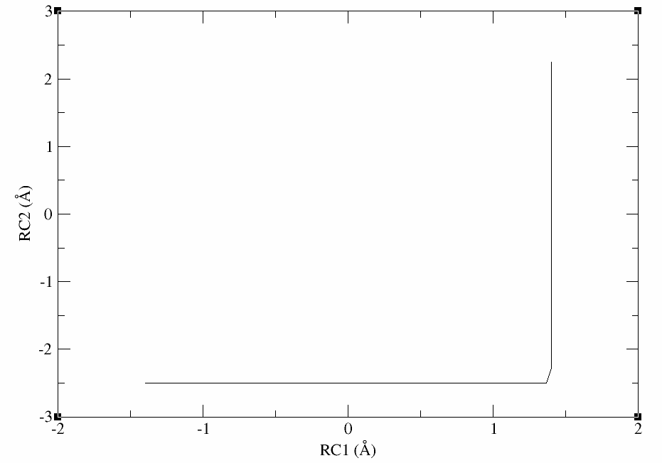
Copy the reaction coordinates to a file called sims.txt and plot them in xmgrace to verify that you have generated a guess where proton transfer preceeds methyl transfer. The file should look like this:
1    -1.400    -2.500   ../equil/img001.disang
2    -1.148    -2.500   ../equil/img002.disang
3    -0.897    -2.500   ../equil/img003.disang
4    -0.645    -2.500   ../equil/img004.disang
5    -0.394    -2.500   ../equil/img005.disang
6    -0.142    -2.500   ../equil/img006.disang
7     0.110    -2.500   ../equil/img007.disang
8     0.361    -2.500   ../equil/img008.disang
9     0.613    -2.500   ../equil/img009.disang
10     0.865    -2.500   ../equil/img010.disang
11     1.116    -2.500   ../equil/img011.disang
12     1.368    -2.500   ../equil/img012.disang
13     1.400    -2.281   ../equil/img013.disang
14     1.400    -2.029   ../equil/img014.disang
15     1.400    -1.777   ../equil/img015.disang
16     1.400    -1.526   ../equil/img016.disang
17     1.400    -1.274   ../equil/img017.disang
18     1.400    -1.023   ../equil/img018.disang
19     1.400    -0.771   ../equil/img019.disang
20     1.400    -0.519   ../equil/img020.disang
21     1.400    -0.268   ../equil/img021.disang
22     1.400    -0.016   ../equil/img022.disang
23     1.400     0.235   ../equil/img023.disang
24     1.400     0.487   ../equil/img024.disang
25     1.400     0.739   ../equil/img025.disang
26     1.400     0.990   ../equil/img026.disang
27     1.400     1.242   ../equil/img027.disang
28     1.400     1.494   ../equil/img028.disang
29     1.400     1.745   ../equil/img029.disang
30     1.400     1.997   ../equil/img030.disang
31     1.400     2.248   ../equil/img031.disang
32     1.400     2.500   ../equil/img032.disang
xmgrace -block sims.txt -bxy 2:3
The plot should look something like this:
Now you would be ready to equilibrate the windows before performing SASM path-finding.
The outputs can be downloaded here:
Attention
5.5. Introduction to running SASM simulations
Under the time constraints of this exercise, the simulation data has been provided for you, and you will perform analysis. The structure files have been ommitted for the sake of file size. First, let’s take a look at how the data was generated.
Chose one of the paths to work with for the exercise (PT, MT, or linear). For the sake of demonstration the activity will follow the linear directory.
cd linear
ls
Example2d.py      analysis.008.log  analysis.019.log  analysis.030.log  analysis.041.log  init   it011  it022  it033  it044
Make2dMovie.sh    analysis.009.log  analysis.020.log  analysis.031.log  analysis.042.log  it001  it012  it023  it034  it045
SASM.slurm        analysis.010.log  analysis.021.log  analysis.032.log  analysis.043.log  it002  it013  it024  it035  it046
analysis.000.log  analysis.011.log  analysis.022.log  analysis.033.log  analysis.044.log  it003  it014  it025  it036  it047
analysis.001.log  analysis.012.log  analysis.023.log  analysis.034.log  analysis.045.log  it004  it015  it026  it037  it048
analysis.002.log  analysis.013.log  analysis.024.log  analysis.035.log  analysis.046.log  it005  it016  it027  it038  it049
analysis.003.log  analysis.014.log  analysis.025.log  analysis.036.log  analysis.047.log  it006  it017  it028  it039  it050
analysis.004.log  analysis.015.log  analysis.026.log  analysis.037.log  analysis.048.log  it007  it018  it029  it040  it051
analysis.005.log  analysis.016.log  analysis.027.log  analysis.038.log  analysis.049.log  it008  it019  it030  it041  it052
analysis.006.log  analysis.017.log  analysis.028.log  analysis.039.log  analysis.050.log  it009  it020  it031  it042  mystring.32.groupfile
analysis.007.log  analysis.018.log  analysis.029.log  analysis.040.log  analysis.051.log  it010  it021  it032  it043  template
In the simulation directory, there is a script called SASM.slurm that was used to generate the data provided to you. The script was set up to run 51 iterations of the string method, each simulation for 4 ps. We will briefly take a look at key lines in the file that are fundamental to using the SASM. First,
MAKEANA="ndfes-path-analyzesims.py --curit=${cit} -d ${DISANG} ${NEQIT} ${TEMP} --maxeq=0.25 --skipg"
Once you have run a set of simulations, this command acts a wrapper for ndfes-CheckEquil.py, ndfes-PrepareAmberData.py, and ndfes-CombineMetafiles.py. It will determine the equilibration region of the simulations up to a fraction of maxeq, and analyze the dumpave files in that region. The resulting metafile will contain data from the current string and previous string iterations, excluding NEQIT iterations. Next, the combined metafile is used to generate the chk file:
MAKECHK="ndfes_omp --mbar -w 0.15 --nboot 0 -c metafile.all.chk metafile.all"
This command remains the same from the 1D example we did previously. Finally, the next string iteration directory is generated using the following command:
MAKESIMS="ndfes-path_omp --curit=${cit} -d ${DISANG} -i ${MDIN} ${NEQIT} ${TEMP} --sasm --maxit=300 --minsize=10 --akima --npathpts=100 --wavg=4 --wavg-niter=1"
This ndfes command optimizes the path on the existing free energy surface in order to determine where the next set of umbrella centers should be placed. The optimization is done by performing up to maxit so called “synthetic iterations” of the string method using npathpts. This optimization essentially decouples the minimum free energy path from the simulated umbrella centers so that the path can be more rigorously represented, and the simulations are performed to improve the quality of sampling. The minsize parameter indicates that a bin should have at least 10 samples to be included in the analysis. The parameter wavg is the order of the cardinal B-spline used to approximate the free energy surface as a weighted average of nearby bin values. The wavg-niter parameter applies an iterative correction to the wavg histogram values such that the interpolated values match the values at the bin centers. Increasing this value will decrease artifacts from averaging, but it may lead to noisier data. These values can be adjusted based on the system and desired smoothness of the free energy surface. Based on the optimized path, the MAKESIMS command will determine the next set of umbrella centers, and it will set up the next run directory based on the template input file and disang file provided.
5.6. Analyzing a set of strings
Now that you understand how the data was generated, you will see how the string has progressed and the resulting free energy surface. The output of the string simulations has been provided for you.
The outputs contain iterations zero (init) through 20, and each iteration contains a directory called analysis. For the init, it002, it005, it010, and it020 directories, the analysis directory has been moved to analysis-out so that you can generate analysis on your own without writing over files, and if you encounter issues, the intended results are still available for you to look at. For the sake of file size, structure files have been removed, but would have been generated by the simulations. For each of these directories you will run the following series of commands. In each case, replace the –curit flag and change the cd command to the directory you are analyzing. When running Example2d.py, change the title to match the iteration, and use the flag –inset-bright instead of –inset-tleft if you are analyzing the MT initial guess of the path.
Check the equilibration, and create the new dumpave files and metafile:
ndfes-path-analyzesims.py --curit=0 -d template/img.disang --neqit=4 --temp=298 --maxeq=0.25 --skipg
Go to the analysis directory
cd init/analysis
Create the chk file:
ndfes_omp --mbar -w 0.15 --nboot 0 -c metafile.all.chk metafile.all
Optimize the path on the free energy surface:
ndfes-path_omp --ipath metafile.current --chk metafile.all.chk --neqit=4 --temp 298 --maxit=300 --minsize=10 --akima --npathpts=100 --wavg=4 --wavg-niter=1 --opath path
Create an image of the free energy surface and current estimate of the path:
python ../../Example2d.py --ipath path.wavg.0.dat --title 'init' --inset-tleft --zerobypath0 --wavg=4 --wavg-niter=1 --minene=-25 --maxene=25 --minsize=10 metafile.all.chk
The ndfes-path-analyzesims.py and ndfes_omp commands are the same as in the SASM run script. For each window, the ndfes-path-analyzesims.py script will print some information about the equilibration of the window. More information can be found by running:
ndfes-CheckEquil.py -h
     Ninp:  The number of input samples
     Nout:  The number of output samples
     Teq:   The percentage of samples excluded as equilibration
     i0:    The 1-based index of the first frame to write (the "start" value
            when using cpptraj)
     s:     The stride through the data (the "offset" value when using cpptraj)
     g:     The statistical inefficiency of the correlated samples
     Wf:    The mean value of the bias potential from the first half of
            statistically independent samples after excluding the first
            i0-1 samples as equilibration
     dWf:   The standard error of Wf
     Wl:    The mean value of the bias potential from the last half of
            statistically independent samples after excluding the first
            i0-1 samples as equilibration
     dWl:   The standard error of Wl
Here we are modifying the ndfes-path_omp command to simply print the minimum free energy path without creating a new simulation directory. Finally, the Example2d.py script will create a figure of the free energy surface with the current estimate of the minimum free energy path and free energy profile. The Example2d.py script as well as a 3d version are available with the ndfes package in the examples directory if you wish to make figures like this for your own projects in the future. If you are unable to obtain the desired output, the files are available in a directory called analysis-out in each of the unanalyzed iteration directories.
Transfer the png files to your local machine
Take a look at the progression of the string by opening metafile.all.chk.wavg.0.path.png for the init, it002, it005, it010, and it020 directories.
For the linear guess, the progression looks something like this:
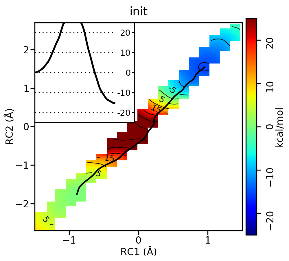
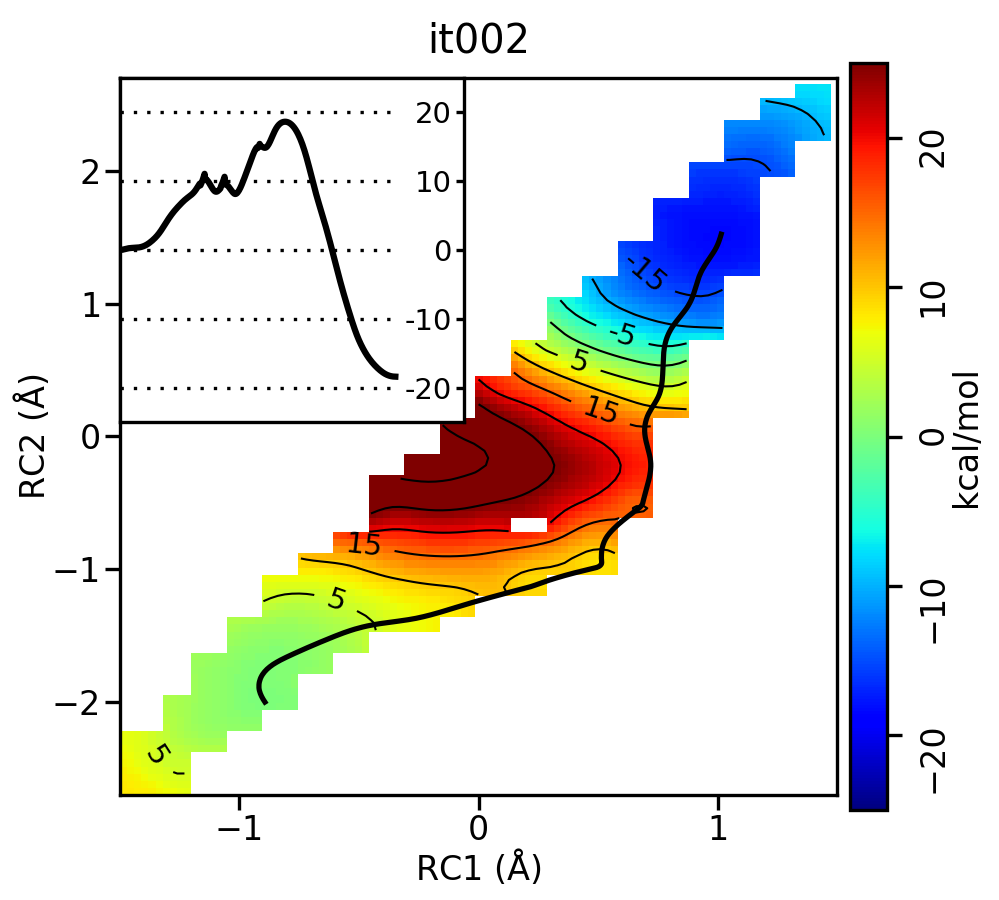
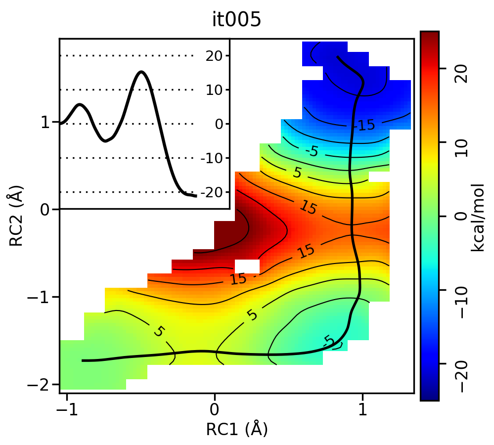
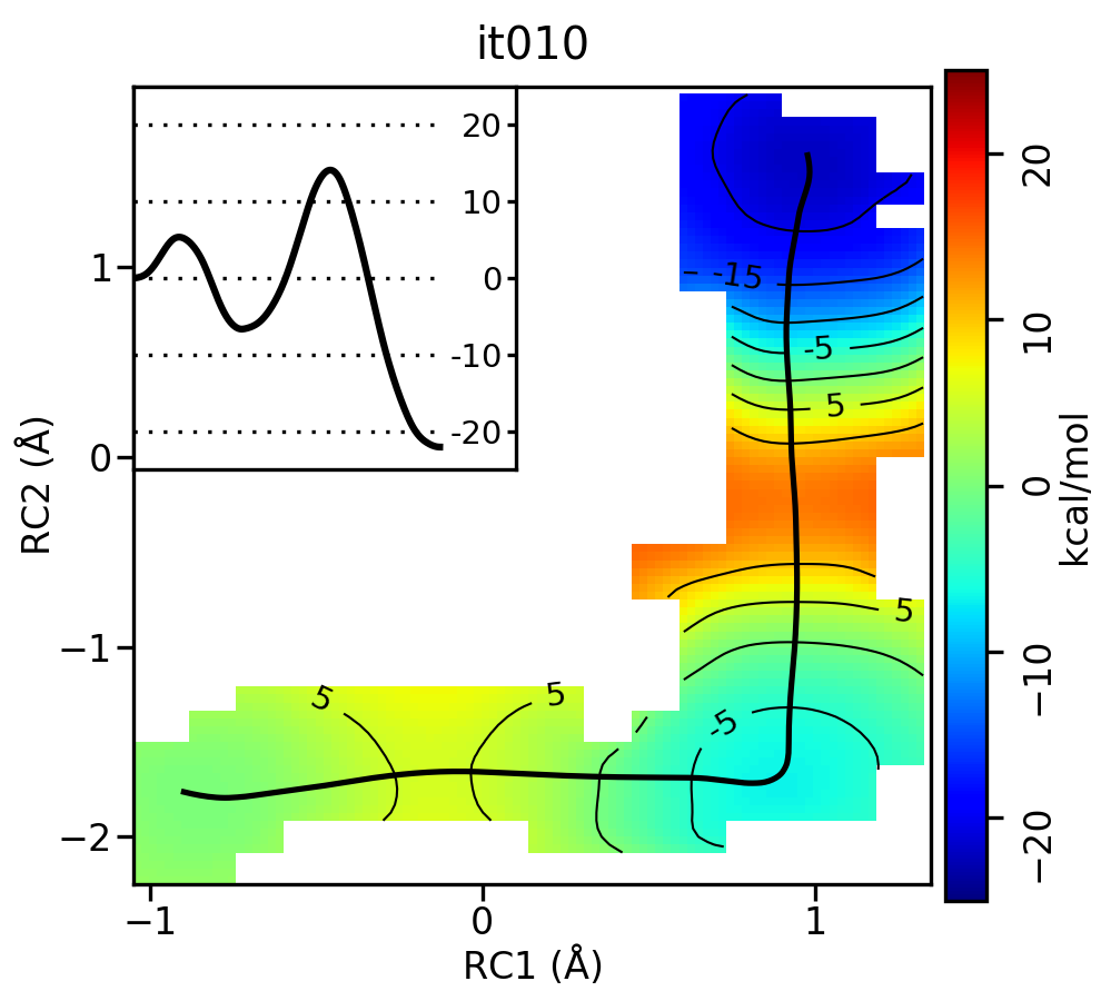
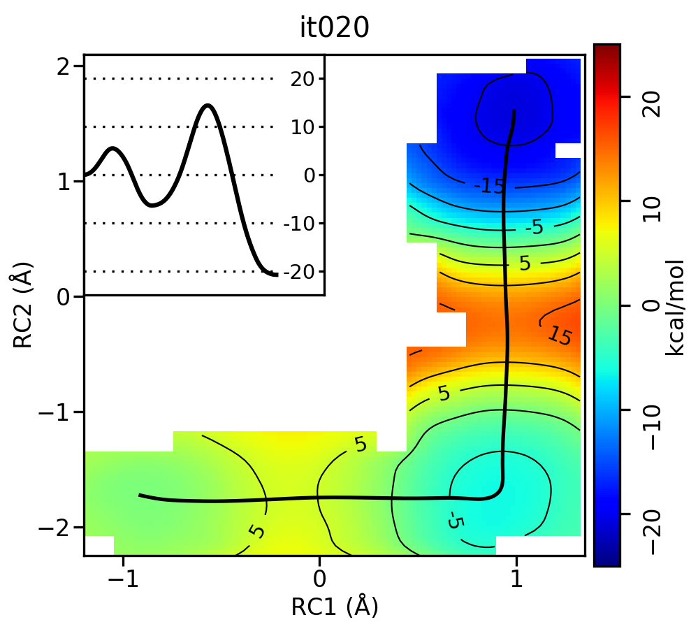
Free energy surfaces starting from a linear initial guess with optimized minimum free energy path (black) after iterations 0, 2, 5, 10, and 20. The inset shows the corresponding PMF.
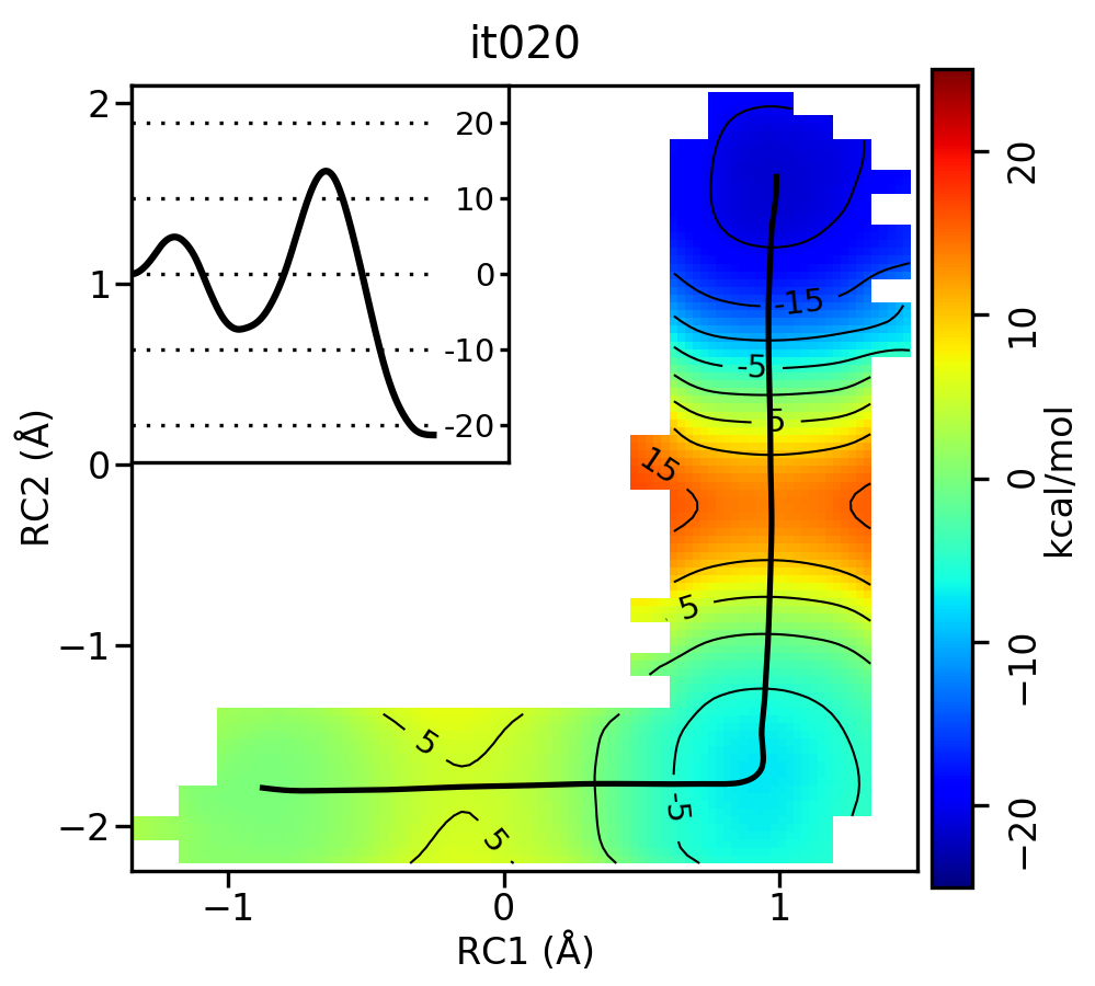
Now let’s compare the path from the different starting guesses. Here is an example of the result from it020 of the strings initiated from the 3 different pathways:
5.6.1. Linear pathway

5.6.2. Stepwise (PT) pathway
5.6.3. Stepwise (MT) pathway
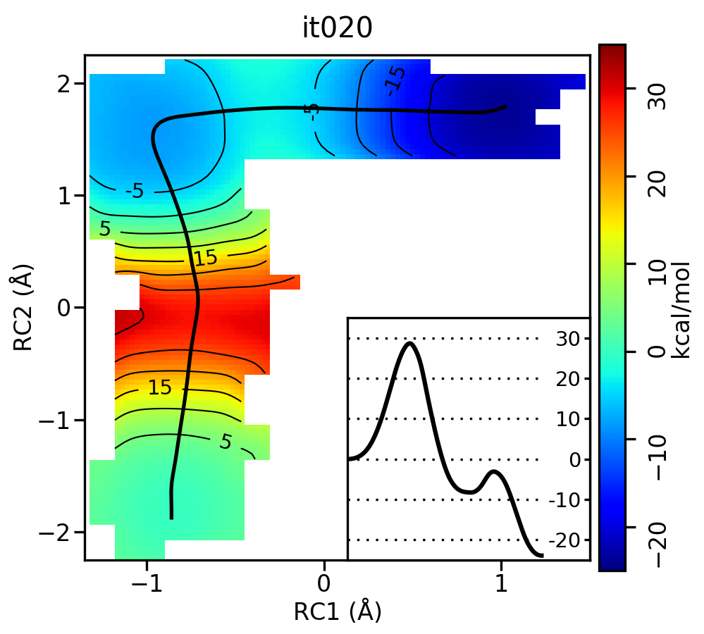
Free energy surfaces starting from a linear and two different step-wise initial guesses with optimized minimum free energy path from 20 string iterations (black). The inset shows the corresponding PMF.
We see that both the linear and stepwise initial guess where proton transfer (RC1) precedes methyl transfer (RC2) both converge to the minimum free energy path, but the stepwise initial guess where methyl transfer precedes proton transfer remains in that local minimum. This highlights that while the SASM is robust, like all string methods one should make educated, and potentially mulitple, initial guesses.
5.7. Visualizing the path progression
Finally, let’s take a look at the convergence of the string over all of the iterations of string data provided in the outputs for the pathway you have chosen (linear, PT, or MT). The Example2d.py script has a feature for creating movies of the string and free energy surface progression. Each string directory contains a script called Make2dMovie.sh that runs the Example2d.py script in order to create a series of png files that are combined into a movie using ffmpeg. This exercise was performed on 50 string iterations to confirm convergence of the path. A run of this script has already been performed for you, and the output was written to the fullmovie directory:
ls fullmovie
movie.sims.mp4  sims.00006.png  sims.00012.png  sims.00018.png  sims.00024.png  sims.00030.png  sims.00036.png  sims.00042.png  sims.00048.png
sims.00001.png  sims.00007.png  sims.00013.png  sims.00019.png  sims.00025.png  sims.00031.png  sims.00037.png  sims.00043.png  sims.00049.png
sims.00002.png  sims.00008.png  sims.00014.png  sims.00020.png  sims.00026.png  sims.00032.png  sims.00038.png  sims.00044.png  sims.00050.png
sims.00003.png  sims.00009.png  sims.00015.png  sims.00021.png  sims.00027.png  sims.00033.png  sims.00039.png  sims.00045.png  sims.00051.png
sims.00004.png  sims.00010.png  sims.00016.png  sims.00022.png  sims.00028.png  sims.00034.png  sims.00040.png  sims.00046.png  sims.00052.png
sims.00005.png  sims.00011.png  sims.00017.png  sims.00023.png  sims.00029.png  sims.00035.png  sims.00041.png  sims.00047.png  sims.00053.png
Transfer the movie.sims.mp4 to your local computer and open the file in google chrome or a supported media player:
google-chrome fullmovie/movie.sims.mp4
Here is the movie depicting the string progression from the linear initial guess:
In the movie, you will see small circles along the path that represent the control points defining the path. The x’s indicate where the umbrella centers have been placed for simulations. You will notice that there is alternation between simulations (x’s) being placed explicitly on the path for refinement and off the path for exploration. This allows for rapid convergence as well as rigorous sampling on both sides of the path. Since we used the neqit=4 flag when running ndfes, string iterations 0-4 are eventually phased out once at least 5 previous iterations of sampling available to analyze. The reasoning is that the initial guess is very poor (the string evolves dramatically), so the short amount of sampling of these early iterations likely do not well-represent an equilibrium ensemble. Feel free to look at the movies generated for the other 2 paths to compare.
Visually, there is very little evolution of the minimum free energy path past iteration 10 or so. When the simulation data was generated, the MAKESIMS command in SASM.slurm outputs two convergence tests to analysis.CIT.log, where CIT is the current iteration. The first test is called the slope test that checks whether the slope of the reaction coordinates over at least 5 iterations is less than the threshold value. The RMSD test checks whether the RMSD of the overall path over at least 5 iterations in less the the threshold value. These are thresholds that have been established based on various test cases, but one should still visually inspect the path.
Check the convergence tests using the following commands:
grep -r "Slopes appear to be converged" *log | head -n5
analysis.008.log:Slopes appear to be converged
analysis.009.log:Slopes appear to be converged
analysis.010.log:Slopes appear to be converged
analysis.011.log:Slopes appear to be converged
analysis.012.log:Slopes appear to be converged

grep -r "Path is effectively CONVERGED" *log
analysis.010.log:Min slope in RMSD    1.687e-03 Path is effectively CONVERGED
analysis.011.log:Min slope in RMSD    6.127e-04 Path is effectively CONVERGED
analysis.012.log:Min slope in RMSD    2.864e-04 Path is effectively CONVERGED
analysis.013.log:Min slope in RMSD    2.337e-04 Path is effectively CONVERGED
analysis.014.log:Min slope in RMSD   -9.001e-05 Path is effectively CONVERGED
Based on this criteria, it appears that both tests were passed by iteration 10 for the linear initial guess. This is consistent with our visual inspection of the movie. Based on the string simulations performed in this activity, it is clear that the minimum free energy path for the MTR1 reaction involves a stepwise mechanism where a general acid protonates the bound ligand to initiate methyl transfer to the target adenine. This free energy barrier (~20 kcal/mol) is about 10 kcal/mol lower than the 1 dimensional case that we computed previously for just methyl transfer, and the 2 dimensional path where methyl transfer precedes proton transfer.
5.8. Comparing the DFTB3 result to the ΔMLP grid
In the previous exercise you analyzed the same reaction sampled on a regular grad. Now we will use SASM to optimize the path on that grid so that we can compare our DFTB3 2D result with the ΔMLP. We will use the MFEP obtained with DFTB3 to optimize the path on the grid. Navigate to the Grid directory:
cd HandsOn5-String/Grid/analysis
ls
Example2d.py  metafile.chk  metafile.string
metafile.string is the metafile from the final iteration of the string departed from the linear guess. Optimize the path on the grid surface and overlay it onto the grid image:
ndfes-path_omp --ipath metafile.string --chk metafile.chk --neqit=4 --temp 298 --maxit=300 --minsize=10 --akima --npathpts=100 --wavg=4 --wavg-niter=1 --opath path
python Example2d.py metafile.chk --xlabel 'PT' --ylabel 'MT' --title '2D grid' --minsize 20 --ipath path.wavg.0.dat
You should have produced metafile.chk.rbf.0.path.png, which looks like this:
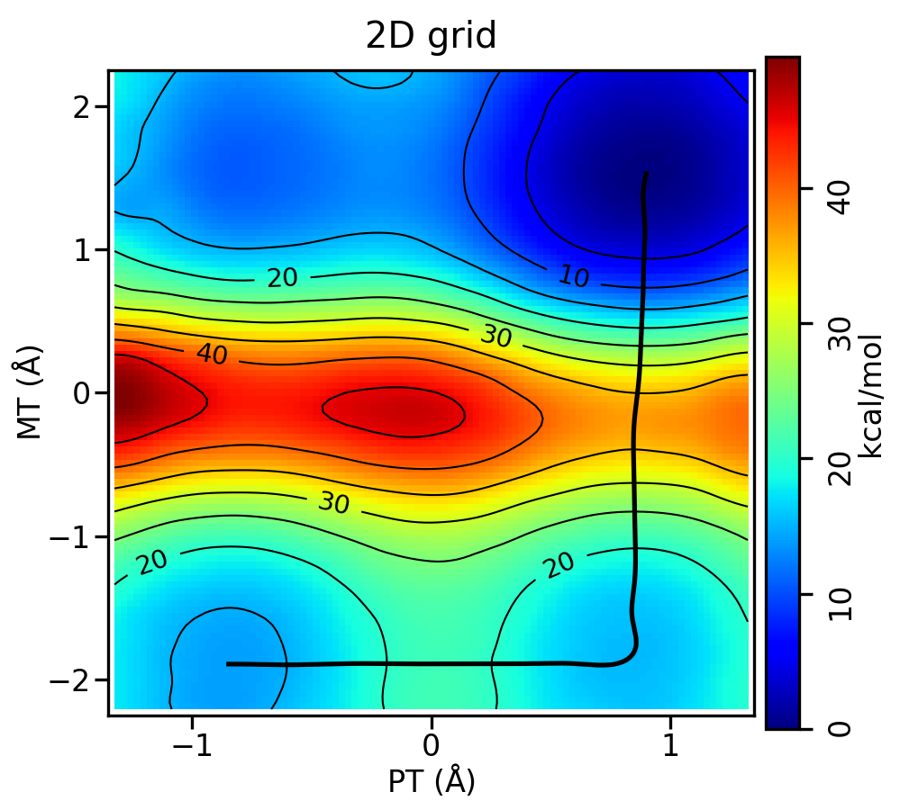
Compared to the DFTB3 free energy surface, the relative free energy of the reactant and intermediate look very similar, while the DFTB3 result has a deeper minima at the intermediate. Plot the resulting PMFs to see the difference between the DFTB3 and ΔMLP PMFs in 2 dimensions:
xmgrace -block path.wavg.0.dat -bxy 2:5 -block ../../linear/it051/analysis/path.032.opt.dat.wavg.0.dat -bxy 2:5
The plot should look something like this:
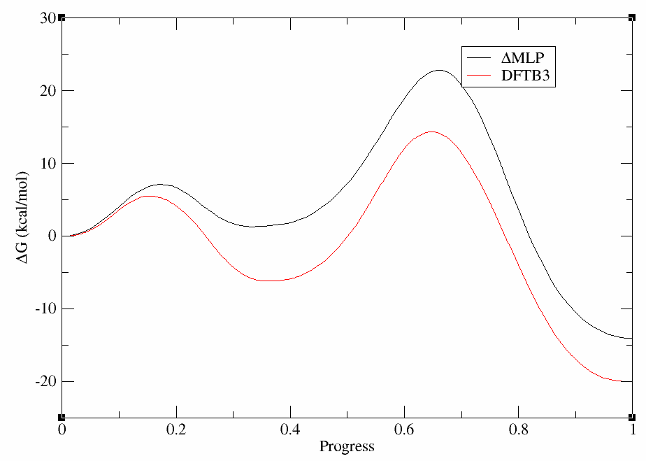
Not only are the rate determining free energy barriers different, but the mechanistic interpretation is different when the higher level of theory is used. At the DFTB3 level (red) there is a stable intermediate state in which the proton transfer has occurred. This would suggest a proton would reside on the ligand a majority of the time. This is contrary to experimental activity-pH profiles of this type of base pair. At the ΔMLP level (black), the intermediate is slightly higher in energy than the reactant state, suggesting the proton would likely be in rapid equilibrium between the cytosine residue and the ligand. This has implications for how one would interpret experimental observables such as pH dependence and highlights the importance of balancing the speed of the simulations with the accuracy of Hamiltonian.
The outputs can be downloaded here:
Attention
5.9. Additional exercise: bootstrap error analysis
Attempt this section if you have extra time after completing the core module. In this section you will learn how to use the bootstrapping functionality in NDFES to compute standard error bars for your PMF after performing SASM pathfinding.
Bootstrapping is an approach for estimating the distribution of a data set by resampling the data with replacement. Performing a “resample” means drawing a sample from the distribution with replacement to form a new data set (ie the new dataset could contain repeats). In this case, our data set is a dumpave file for a simulation. If we perform 50 boostraps, we will obtain 50 variations of the dumpave file. This assumes that all samples are statistically independent. If not, NDFES will compute the autocorrelation time in the dataset and samples will consist of blocks where the stride is the statistical inefficiency. In that case, blocks are drawn as samples rather than single values. From the resampled data sets, we can compute the standard error.
The suggested approach for computing error bars with NDFES combines bootstrapping and ensemble averaging. This requires that one perform multiple trials, and perform bootstrapping for each one. The final error estimate incorporates the average variance in the bootstrap uncertainties and the variance between trials. For more information on this approach, please see refer to the NDFES documentation.
You have been provided the directory called ErrorAnalysis where 4 trials of production sampling have been performed for you. To speed up the bootstrapping, only 5 ps of sampling have been performed, but it is best practice to perform more to obtain convergence. These are 4 independent production trials initiated from simulations with different random seeds on the final converged path from the linear guess SASM simulations. Navigate to the ErrorAnalysis directory:
cd ErrorAnalysis
ls
tr1 tr2 tr3 tr4 Analysis

cd Analysis
ls
analyze.sh
Here are the contents of analyze.sh:
#!/bin/bash

export OMP_NUM_THREADS=4

top=`pwd`

## Create a chk file for each trial

for dir in tr1 tr2 tr3 tr4; do

    cd ../${dir}

    if [[ ! -d "analysis" ]]; then
        mkdir analysis
        mkdir analysis/dumpaves
    fi

    cd analysis

    if [[ -f "metafile" ]]; then
        rm metafile
    fi

    for i in $(seq 1 32); do
      base=$(printf "img%02i" ${i})
      ndfes-PrepareAmberData.py -d ../${base}.disang -i ../${base}.dumpave -o dumpaves/${base}.dumpave -r 1 >> metafile
    done

    ndfes_omp --mbar -w 0.15 --nboot 50 -c metafile.chk metafile ## Use nboot=50 to perform 50 bootstrap resamples
    cp metafile.chk ${top}/Analysis/metafile.${dir}.chk

    cd ${top}

done

## This defines the path
cp ../tr1/metafile.current ./

## Combine the metafiles
ndfes-CombineMetafiles.py ..tr{1..4}/analysis/metafile --out metafile

## Obtain the combined free energy surface (this is what we want the PMF to be computed on)
ndfes_omp --mbar -w 0.15 --nboot 50 -c metafile.chk metafile

## Get the PMF along the path on the combined free energy surface
ndfes-path_omp --chk metafile.chk --ipath metafile.current --npathpts 32 --nsplpts 100 --opath path --wavg=4 --wavg-niter=1 --minsize=10

## Read the free energy from the combined surface (--ene), but average the bootstrap errors from 4 trials
ndfes-AvgFESs.py --ene metafile.chk --fes metafile.tr1.chk=0 --fes metafile.tr2.chk=0 --fes metafile.tr3.chk=0 --fes metafile.tr4.chk=0 --out avg.chk

## Get the path along the combined surface but with bootstrap errors averaged over the trials
ndfes-path_omp --chk avg.chk --ipath path.wavg.0.dat --npathpts 32 --nsplpts 100 --opath path.avg --wavg=4 --wavg-niter=1 --minsize=10
First you will compute the free energy surface for each trial and compute the associated bootstrap standard errors (accomplished by the for loop). Then you will generate the aggreagte free energy surface from the 4 trials. This is the free energy surface from which you want to obtain the final free energy profile. Next you use the ndfes-AvgFESs.py functionality to compute the standard error of an average free energy surface computed from samples that have their own error estimates. This requires that the free energies from each trial be aligned. This is accomplished by computing a set of constants that minimizes the weighted sum of squared error to a reference surface. Once the surfaces are aligned, the combined error estimate is computed.
Run analyze.sh:
bash analyze.sh 2>&1 | tee bootstrap.out
Let’s break down some of the output written to bootstrap.out:
State  Ham       T Ineff       N      X1      K1    <X1>   SD X1      X2      K2    <X2>   SD X2
  idx  idx
    0    0  298.00     2     500   -0.86  100.00   -0.86    0.05   -1.74  100.00   -1.74    0.05
    1    0  298.00     2     500   -0.70  100.00   -0.73    0.05   -1.77  100.00   -1.77    0.05
    2    0  298.00     2     500   -0.53  100.00   -0.58    0.06   -1.78  100.00   -1.78    0.05
    3    0  298.00     6     500   -0.36  100.00   -0.42    0.05   -1.77  100.00   -1.77    0.05
    4    0  298.00     2     500   -0.20  100.00   -0.22    0.06   -1.76  100.00   -1.77    0.05
    5    0  298.00     3     500   -0.03  100.00   -0.00    0.06   -1.75  100.00   -1.76    0.05
    6    0  298.00     3     500    0.14  100.00    0.20    0.06   -1.74  100.00   -1.74    0.05
    7    0  298.00     7     500    0.30  100.00    0.39    0.06   -1.75  100.00   -1.75    0.05
    8    0  298.00     2     500    0.47  100.00    0.55    0.05   -1.75  100.00   -1.76    0.05
    9    0  298.00     2     500    0.64  100.00    0.70    0.06   -1.75  100.00   -1.75    0.05
  10    0  298.00     2     500    0.80  100.00    0.83    0.05   -1.76  100.00   -1.76    0.05
  11    0  298.00     5     500    0.92  100.00    0.93    0.06   -1.67  100.00   -1.67    0.05
  12    0  298.00     7     500    0.93  100.00    0.93    0.05   -1.50  100.00   -1.52    0.06
  13    0  298.00     2     500    0.93  100.00    0.94    0.05   -1.34  100.00   -1.38    0.05
  14    0  298.00     1     500    0.93  100.00    0.94    0.06   -1.17  100.00   -1.24    0.05
  15    0  298.00     1     500    0.94  100.00    0.94    0.05   -1.00  100.00   -1.09    0.05
  16    0  298.00     1     500    0.95  100.00    0.94    0.05   -0.84  100.00   -0.95    0.05
  17    0  298.00     1     500    0.95  100.00    0.95    0.04   -0.67  100.00   -0.80    0.06
  18    0  298.00     1     500    0.95  100.00    0.96    0.05   -0.50  100.00   -0.61    0.06
  19    0  298.00     1     500    0.95  100.00    0.95    0.05   -0.34  100.00   -0.40    0.07
  20    0  298.00     2     500    0.95  100.00    0.95    0.06   -0.17  100.00   -0.16    0.06
  21    0  298.00     1     500    0.95  100.00    0.95    0.05   -0.00  100.00    0.11    0.06
  22    0  298.00     1     500    0.94  100.00    0.94    0.04    0.16  100.00    0.31    0.06
  23    0  298.00     1     500    0.94  100.00    0.94    0.05    0.33  100.00    0.50    0.05
  24    0  298.00     1     500    0.94  100.00    0.93    0.05    0.50  100.00    0.66    0.05
  25    0  298.00     1     500    0.94  100.00    0.94    0.04    0.66  100.00    0.80    0.05
  26    0  298.00     1     500    0.94  100.00    0.94    0.05    0.83  100.00    0.94    0.05
  27    0  298.00     2     500    0.94  100.00    0.94    0.05    1.00  100.00    1.08    0.05
  28    0  298.00     1     500    0.95  100.00    0.95    0.06    1.16  100.00    1.23    0.05
  29    0  298.00     1     500    0.96  100.00    0.96    0.05    1.33  100.00    1.34    0.05
  30    0  298.00     8     500    0.99  100.00    0.98    0.05    1.50  100.00    1.50    0.05
  31    0  298.00     4     500    0.99  100.00    0.99    0.05    1.61  100.00    1.62    0.05
Iter           Objective    Rel Change
    1   -6.6248024323e-01      0.00e+00 *
    2   -6.6361832793e-01     -1.72e-03 *
    3   -1.0030386217e+00     -5.11e-01 *
    4   -1.3344462443e+00     -3.30e-01 *
    5   -1.4979847263e+00     -1.23e-01 *
    6   -1.5655918218e+00     -4.51e-02 *
    7   -1.6101936436e+00     -2.85e-02 *
    8   -1.6639555659e+00     -3.34e-02 *
    9   -1.7020658753e+00     -2.29e-02 *
  10   -1.7281001621e+00     -1.53e-02 *
  11   -1.7377016264e+00     -5.56e-03 *
  12   -1.7469957149e+00     -5.35e-03 *
  13   -1.7476228925e+00     -3.59e-04 *
  14   -1.7534916764e+00     -3.36e-03 *
  15   -1.7545582000e+00     -6.08e-04 *
  16   -1.7562398597e+00     -9.58e-04 *
  17   -1.7584692751e+00     -1.27e-03 *
  18   -1.7586464424e+00     -1.01e-04 *
  19   -1.7626023365e+00     -2.25e-03 *
  20   -1.7636118238e+00     -5.73e-04 *
  21   -1.7650481787e+00     -8.14e-04 *
  22   -1.7663867456e+00     -7.58e-04 *
  23   -1.7675032288e+00     -6.32e-04 *
  24   -1.7685237823e+00     -5.77e-04 *
  25   -1.7695153806e+00     -5.61e-04 *
  26   -1.7703095832e+00     -4.49e-04 *
  27   -1.7698563231e+00      2.56e-04
  28   -1.7705513070e+00     -1.37e-04 *
  29   -1.7708645015e+00     -1.77e-04 *
  30   -1.7710267061e+00     -9.16e-05 *
  31   -1.7713033461e+00     -1.56e-04 *
  32   -1.7716516980e+00     -1.97e-04 *
  33   -1.7722472925e+00     -3.36e-04 *
  34   -1.7729957572e+00     -4.22e-04 *
  35   -1.7740398781e+00     -5.89e-04 *
  36   -1.7747003672e+00     -3.72e-04 *
  37   -1.7746151837e+00      4.80e-05
  38   -1.7747875238e+00     -4.91e-05 *
  39   -1.7748407690e+00     -3.00e-05 *
  40   -1.7748471486e+00     -3.59e-06 *
  41   -1.7748481445e+00     -5.61e-07 *
  42   -1.7748486458e+00     -2.82e-07 *
  43   -1.7748486794e+00     -1.89e-08 *
  44   -1.7748487632e+00     -4.72e-08 *
  45   -1.7748487651e+00     -1.07e-09 *
  46   -1.7748487662e+00     -5.95e-10 *
  47   -1.7748487663e+00     -4.78e-11 *
Optimization completed successfully because 'ftol_rel' or 'ftol_abs' was reached
Bootstrap    1 /   50
Bootstrap    2 /   50
Bootstrap    3 /   50
Bootstrap    4 /   50
Bootstrap    5 /   50
Bootstrap    6 /   50
Bootstrap    7 /   50
Bootstrap    8 /   50
Bootstrap    9 /   50
Bootstrap   10 /   50
Bootstrap   11 /   50
Bootstrap   12 /   50
Bootstrap   13 /   50
Bootstrap   14 /   50
Bootstrap   15 /   50
Bootstrap   16 /   50
Bootstrap   17 /   50
Bootstrap   18 /   50
Bootstrap   19 /   50
Bootstrap   20 /   50
Bootstrap   21 /   50
Bootstrap   22 /   50
Bootstrap   23 /   50
Bootstrap   24 /   50
Bootstrap   25 /   50
Bootstrap   26 /   50
Bootstrap   27 /   50
Bootstrap   28 /   50
Bootstrap   29 /   50
Bootstrap   30 /   50
Bootstrap   31 /   50
Bootstrap   32 /   50
Bootstrap   33 /   50
Bootstrap   34 /   50
Bootstrap   35 /   50
Bootstrap   36 /   50
Bootstrap   37 /   50
Bootstrap   38 /   50
Bootstrap   39 /   50
Bootstrap   40 /   50
Bootstrap   41 /   50
Bootstrap   42 /   50
Bootstrap   43 /   50
Bootstrap   44 /   50
Bootstrap   45 /   50
Bootstrap   46 /   50
Bootstrap   47 /   50
Bootstrap   48 /   50
Bootstrap   49 /   50
Bootstrap   50 /   50
The statistical inefficiency informs how samples will be drawn for bootstrapping. Then after performing MBAR analysis to compute the free energy, 50 bootstrap resamplings are performed.
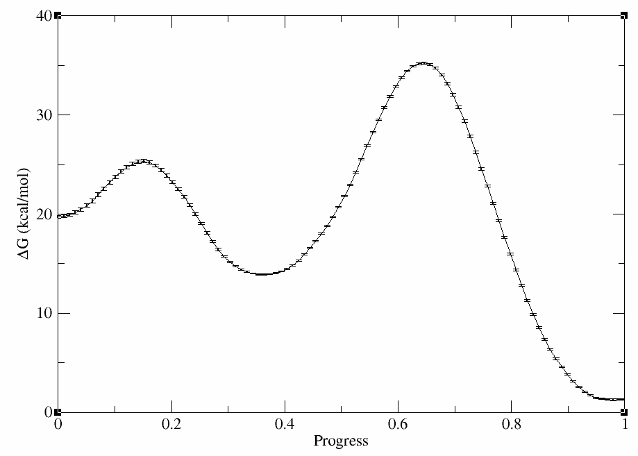
You should have produced path.avg.wavg.0.dat. It should contain 8 columns: index, progress, proton transfer coordinate, methyl transfer coordinate, free energy, bootstrap standard error, reweighting entropy, and the number of samples in the bin that the point is contained in. Plot the free energy profile with error bars using xmgrace:
xmgrace -block path.avg.wavg.0.dat -settype xydy -bxy 2:5:6
The plot should look something like this:
The outputs can be downloaded here:
Attention
5.10. References
McCarthy, E.; Ekesan, Ş; Giese, T. J.; Wilson, T. J.; Deng, J.; Huang, L.; Lilley, D. J.; York, D. M. Catalytic mechanism and pH dependence of a methyltransferase ribozyme (MTR1) from computational enzymology. Nucleic Acids Res. 2023, 51, 4508-4518 (10.1093/nar/gkad260)
Giese, T. J.; Ekesan, Ş; McCarthy, E.; Tao, Y.; York, D. M. Surface-Accelerated String Method for Locating Minimum Free Energy Paths. J. Chem. Theory Comput. 2024, 20, 2058– 2073 ( 10.1021/acs.jctc.3c01401)
Giese, T. J.; Ekesan, Ş; York, D. M. Extension of the Variational Free Energy Profile and Multistate Bennett Acceptance Ratio Methods for High-Dimensional Potential of Mean Force Profile Analysis. J. Phys. Chem. A 2021, 125, 4216– 4232 (10.1021/acs.jpca.1c00736)
Gaus, M.; Cui, Q.; Elstner, M. DFTB3: Extension of the Self-Consistent-Charge Density-Functional Tight-Binding Method (SCC-DFTB). J. Chem. Theory Comput. 2011, 7, 931– 948 (10.1021/ct100684s)