2. Hands-On Session 2: Introduction to Molecular Dynamics Simulations with Amber
2.1. Learning Objectives
Understand the basic workflow of molecular dynamics (MD) simulations using AMBER, from equilibration to production.
Perform stepwise equilibration, apply and gradually release positional restraints during equilibration.
Read and modify AMBER input files (.mdin) for common MD stages (minimization, heating, equilibration, production).
Use cpptraj to process MD outputs and prepare structures for visualization.
Visualize MD results with VMD and compare structures before and after equilibration.
Understand the special considerations made to stably equilibrating a nucleic acid system.
2.2. Relevant Literature
The following references provide background and context for the methods and best practices used in this activity:
McCarthy, E.; Ekesan, Ş.; Giese, T. J.; Wilson, T. J.; Deng, J.; Huang, L.; Lilley, D. J.; York, D. M. Catalytic mechanism and pH dependence of a methyltransferase ribozyme (MTR1) from computational enzymology. Nucleic Acids Research 2023, 51, 4508–4518. (https://doi.org/10.1093/nar/gkad260)
Deng, J.; Wilson, T. J.; Wang, J.; Peng, X.; Li, M.; Lin, X.; Liao, W.; Lilley, D. M. J.; Huang, L. Structure and mechanism of a methyltransferase ribozyme. Nature Chemical Biology 2022, 18, 556–564. (https://doi.org/10.1038/s41589-022-00982-z)
Zgarbová, M.; Otyepka, M.; Šponer, J.; Mládek, A.; Banáš, P.; Cheatham, T. E., III; Jurečka, P. Refinement of the Cornell et al. nucleic acids force field based on reference quantum chemical calculations of glycosidic torsion profiles. Journal of Chemical Theory and Computation 2011, 7, 2886–2902. (https://doi.org/10.1021/ct200162x)
Horn, H. W.; Swope, W. C.; Pitera, J. W.; Madura, J. D.; Dick, T. J.; Hura, G. L.; Head-Gordon, T. Development of an improved four-site water model for biomolecular simulations: TIP4P-Ew. Journal of Chemical Physics 2004, 120, 9665–9678. (https://doi.org/10.1063/1.1683075)
2.3. Activities
        flowchart LR

%% =========================
%% Equilibration
%% =========================

A2["Input files<br/>MTR1_counterIon_water_bulk.parm7"]

A1["Input files<br/>MTR1_counterIon_water_bulk.rst7<br/>mdins/*.mdin<br/>restrnt.disang"]

P1{{"<b>[§2.3.4.2]</b><br/>Run equilibration<br/>sander / pmemd.cuda"}}

O1_1["<b>[from §2.3.4.2]</b><br/>Equilibration outputs<br/>mdout<br/>equil.nc<br/>"]

O1_2["<b>[from §2.3.4.2]</b><br/>Final restart<br/>09_Equil_solute_Rwt2-run.rst7"]

A1 --> P1
A2 --> P1
P1 --> O1_1
P1 --> O1_2


%% =========================
%% Wrap equilibrated restart and trajectory
%% =========================

P2{{"<b>[§2.3.4.3]</b><br/>Wrap equilibration<br/>cpptraj"}}

O2["<b>[from §2.3.4.3]</b><br/>Wrapped equilibration files<br/>centered.09_Equil_solute_Rwt2-run.rst7<br/>centered_equil.nc"]

O1_1 --> P2
O1_2 --> P2
P2 --> O2


%% =========================
%% Inspect equilibration
%% =========================

P3{{"<b>[§2.3.4.3]</b><br/>Inspect equilibration<br/>VMD"}}

O3["Equilibration inspection<br/>RNA RMSD<br/>ion positions"]

O2 --> P3
P3 --> O3


%% =========================
%% Prepare and Run Production
%% =========================

P4{{"<b>[§2.3.5.2]</b><br/>Apply HMR<br/>cpptraj"}}
O4["<b>[from §2.3.5.2]</b><br/>HMR topology<br/>MTR1_counterIon_water_bulk-run.parm7"]

A2 --> P4
P4 --> O4


P5{{"<b>[§2.3.5.3]</b><br/>Run production MD<br/>pmemd.cuda"}}
O5_1["<b>[from §2.3.5.3]</b><br/>Production logs<br/>MTR1_counterIon_water_bulk-run-01.mdout<br/>MTR1_counterIon_water_bulk-run-01.mdinfo"]

O5_2["<b>[from §2.3.5.3]</b><br/>Production trajectory/restart<br/>MTR1_counterIon_water_bulk-run-01.nc<br/>MTR1_counterIon_water_bulk-run-01.rst7"]


O1_2 --> P5
O4 --> P5
P5 --> O5_1
P5 --> O5_2

P6{{"<b>[§2.3.5.4]</b><br/>Wrap production<br/>cpptraj"}}
O6["<b>[from §2.3.5.4]</b><br/>Wrapped production files<br/>centered.MTR1_counterIon_water_bulk-run-01.nc<br/>centered.MTR1_counterIon_water_bulk-run-01.rst7"]

O5_2 --> P6
P6 --> O6

O7["Production inspection<br/>RNA RMSD<br/>ion positions"]

P7{{"<b>[§2.3.5.4]</b><br/>Inspect production<br/>VMD"}}
O6 --> P7
P7 --> O7

%% =========================
%% Styling
%% =========================

classDef file fill:#fff7e6,stroke:#d98c00,stroke-width:1.5px,color:#111;
classDef program fill:#e8f1ff,stroke:#1f77b4,stroke-width:1.8px,color:#111;
classDef result fill:#eaf7ea,stroke:#2ca02c,stroke-width:1.5px,color:#111;

class A1,A2 file;
class P1,P2,P3,P4,P5,P6,P7 program;
class O1_1,O1_2,O2,O3,O4,O5_1,O5_2,O6,O7 result;
2.3.1. Starting structure and input files
This activity starts from pre-generated AMBER topology and coordinate files that define the initial structure of the fully solvated RNA system with counterions. These files serve as the starting point for all subsequent equilibration and production molecular dynamics simulations performed in this activity.
Starting from these files, the system will be equilibrated stepwise and then used to run production molecular dynamics simulations, generating new restart and trajectory files at each stage.
The specific starting files used in this activity are:
These files ar used to demonstrate the complete equilibration and production molecular dynamics workflow.
2.3.2. Accessing the activity files
All input files and reference output files required for this activity are provided in two ways.
Option 1: On the cluster
For convenience during the workshop, the full directory associated with Hands-On Session 2 is already available on the cluster and can be copied directly to your working directory from:
/path/Day1/HS2/Files
This directory contains all input files as well as reference output files corresponding to the equilibration and production steps described in this activity.
Option 2: Downloadable archive
All input files and reference output files can also be downloaded as a single compressed archive:
2.3.3. Equilibration and Production Workflow
        flowchart LR

A["Initial system<br/>Inputs: parm7, rst7 (ions and solvent)"]

subgraph EQ["Equilibration"]
   direction LR
   B["Solvent equilibration<br/>Restrained solute"]
   C["Heating to 300 K"]
   D["Gradual solute release"]
   E["Wrap and inspect equilibration<br/>Centered equilibration structure"]
   B --> C --> D --> E
end

subgraph PR["Production"]
   direction LR
   F["Production MD<br/>Unrestrained system"]
   G["Wrap and inspect production<br/>Centered production trajectory"]
   F --> G
end

subgraph AN["Analysis"]
   direction LR
   H["Final inspection and analysis<br/>RMSD, visualization"]
end

A --> B
E --> F
G --> H
2.3.4. Equilibrating the Box
Copy the inputs to your working directory:
mkdir MTR1_Equil
cd MTR1_Equil
cp -r /path/Day1/HS2/Files/input/Equil/* ./
Now you will learn how to equilibrate the simulation box. Electrostatic interactions are extremely important for RNA structure given the negatively charged backbone. Therefore, a rigorous equilibration process allows the solvent to properly organize around the molecule in a controlled way while avoiding large fluctuations in density that could cause errors. This is especially important when your system contains divalent metal ions. The electrostatic interaction energy is proportional to the product of the two charges, so increasing the charge will lead to a larger interaction energy at a given distance. Nucleic acids are highly charged systems and must be equilibrated slowly.
You have been provided the Equil directory containing
eqFromStratch.slurm and a directory called mdins.
List the contents of the mdins directory:
ls mdins
000_Min.mdin  003_NPT.mdin  03_Equil_NPT_solvent.mdin  06_Equil_solute_Rwt25.mdin  09_Equil_solute_Rwt2.mdin
001_NPT.mdin  01_Min.mdin   04_Min_solute.mdin         07_Equil_solute_Rwt10.mdin
002_NPT.mdin  02_Heat.mdin  05_Heat_solute_Rwt25.mdin  08_Equil_solute_Rwt5.mdin
These are the input files for the stepwise equilibration procedure and subsequent production simulation.
Note
The general approach is to slowly equilibrate the solvent around the solute, then gradually allow the solute to move. We cycle through minimizations to remove clashes and find a local minimum, heating to explore new conformations, then simulations in the NPT ensemble to approach the global minimum. There are some specific points to note about how the provided mdin files have been written.
2.3.4.1. Equilibration input files
Initial energy minimization of the solvent. Solute atoms are positionally restrained with weights of 50 kcal/mol Ų.
The line highlighted in the initial minimization input file specifies the positional restraint mask used during equilibration. Restraints are applied to all atoms that are not hydrogens and not part of the solvent or ions (
NA,CL,MG,WAT). As a result, all heavy atoms of the solute are restrained, while solvent molecules and ions are free to relax. In practice, this effectively keeps the RNA heavy atoms close to their starting positions during the early stages of equilibration. There is no Mg2+ in this system currently, but many RNA systems will contain it. If additional solvent components are present, they should be included in the restraint mask. When ions were added in LEaP they were referred to asNAandCL, but equivalent residue names such asNa+andCl-would also be handled correctly by the mask.Another highlighted line in the same input file indicates that a file named
restrnt.disangis read as input. This file can contain NMR-style restraints, such as distance, angle, or torsion restraints between selected atoms. These restraints differ from coordinate restraints (enabled byntr = 1), as atoms are allowed to fluctuate while maintaining defined geometric relationships.
Initial Solvent Energy Minimization Stage
Bulk water and Sodium ions only

&cntrl
  imin = 1
  ntmin = 0
  maxcyc = 500
  ntx = 1
  ntpr = 250
  ntwx = 0
  ntr = 1
  restraint_wt = 50.0
  restraintmask = '!@H= & !:NA,CL,MG,WAT'
  cut = 12.0
/
&wt type = 'DUMPFREQ', istep1 = 10000, /
&wt type='END' /
DISANG=restrnt.disang
DUMPAVE=restrnt.dumpave
LISTOUT=POUT
LISTIN=POUT
Initial equilibration in the NPT ensemble. Temperature is held at 300 K and pressure at 1 atm for 5 ps. Solute atoms are positionally restrained with weights of 50 kcal/mol Ų.
&cntrl
  imin = 0
  ntx = 1
  nstlim = 2500
  ntb = 2
  ntp = 1
  temp0 = 300.0
  ntr = 1
  restraint_wt = 50.0
  restraintmask = '!@H= & !:NA,CL,MG,WAT'
  cut = 12.0
/
Additional equilibration in the NPT ensemble. Identical to the previous step, but velocities are read to allow gradual box relaxation and avoid large density fluctuations.
&cntrl
  imin = 0
  ntx = 5
  nstlim = 2500
  ntb = 2
  ntp = 1
  temp0 = 300.0
  ntr = 1
  restraint_wt = 50.0
  restraintmask = '!@H= & !:NA,CL,MG,WAT'
  cut = 12.0
/
Extended equilibration in the NPT ensemble. This step is run continuously for 190 ps to complete a total of 200 ps of NPT equilibration.
&cntrl
  imin = 0
  ntx = 5
  nstlim = 95000
  ntb = 2
  ntp = 1
  temp0 = 300.0
  ntr = 1
  restraint_wt = 50.0
  restraintmask = '!@H= & !:NA,CL,MG,WAT'
  cut = 12.0
/
Solvent energy minimization. Solute atoms remain positionally restrained to remove residual clashes after initial equilibration.
&ntrl
  imin = 1
  ntmin = 0
  maxcyc = 500
  ntx = 1
  ntpr = 250
  ntwx = 0
  ntr = 1
  restraint_wt = 50.0
  restraintmask = '!@H= & !:NA,CL,MG,WAT'
  cut = 12.0
/
DISANG=restrnt.disang
Initial heating at constant volume. The temperature is increased from 0 to 300 K over 600 ps and then held constant for 1 ns, with positional restraints applied.
&cntrl
  imin = 0
  ntx = 1
  nstlim = 800000
  dt = 0.002
  ntc = 2
  ntf = 2
  ntb = 1/_static/files/WorkshopTutorials/2026_Amber_Workshop_SSB/Day1/HandsOn2-MD/Files/output/Equil/centered.09_Equil_solute_Rwt2-run.rst7
  ntt = 3
  tempi = 0.0
  temp0 = 300.0
  gamma_ln = 2.0
  ntpr = 500
  ntwx = 500
  ntr = 1
  restraint_wt = 50.0
  restraintmask = '!@H= & !:NA,CL,MG,WAT'
  cut = 12.0
/
Solvent equilibration in the NPT ensemble. Temperature is held at 300 K and pressure at 1 atm for 5 ns while the solute remains restrained.
Download 03_Equil_NPT_solvent.mdin
&cntrl
  imin = 0
  ntx = 5
  nstlim = 2500000
  dt = 0.002
  ntc = 2
  ntf = 2
  ntb = 2
  ntp = 1
  pres0 = 1.0
  taup = 1.0
  ntt = 3
  temp0 = 300.0
  gamma_ln = 2.0
  ntpr = 5000
  ntwx = 5000
  ntr = 1
  restraint_wt = 50.0
  restraintmask = '!@H= & !:NA,CL,MG,WAT'
  cut = 12.0
/
Solute energy minimization. Positional restraints are released to relax the solute and solvent with respect to each other.
&cntrl
  imin = 1
  ntmin = 0
  maxcyc = 500
  ntx = 1
  ntpr = 250
  ntwx = 0
  ntr = 0
  cut = 12.0
/
Solute heating with reduced restraints. Increase the temperature from 0 to 300 K over 600 ps, then hold at constant temperature for 1 ns. Solute atoms are positionally restrained with weights of 25 kcal/mol². The restraints are released gradually over ensuing stages of dynamics. Changing restraints effectively changes the force field. If the energy associated with a restraint is high and it is suddenly removed, the bonds to the associated atom could be broken as the atom position changes dramatically in a step of dynamics.
Download 05_Heat_solute_Rwt25.mdin
&cntrl
  imin = 0
  ntx = 1
  nstlim = 800000
  dt = 0.002
  ntc = 2
  ntf = 2
  ntb = 1
  ntt = 3
  tempi = 0.0
  temp0 = 300.0
  gamma_ln = 2.0
  ntpr = 500
  ntwx = 500
  ntr = 1
  restraint_wt = 25.0
  restraintmask = '!@H= & !:NA,CL,MG,WAT'
  cut = 12.0
/
Solute equilibration with 25 kcal/mol Ų restraints. Short 500 ps NPT equilibration at reduced restraint strength.
Download 06_Equil_solute_Rwt25.mdin
&cntrl
  imin = 0
  ntx = 5
  nstlim = 250000
  dt = 0.002
  ntc = 2
  ntf = 2
  ntb = 2
  ntp = 1
  pres0 = 1.0
  taup = 1.0
  ntt = 3
  temp0 = 300.0
  gamma_ln = 2.0
  ntpr = 5000
  ntwx = 5000
  ntr = 1
  restraint_wt = 25.0
  restraintmask = '!@H= & !:NA,CL,MG,WAT'
  cut = 12.0
/
Solute equilibration with 10 kcal/mol Ų restraints. During 500 ps.
Download 07_Equil_solute_Rwt10.mdin
&cntrl
  imin = 0
  ntx = 5
  nstlim = 250000
  dt = 0.002
  ntc = 2
  ntf = 2
  ntb = 2
  ntp = 1
  pres0 = 1.0
  taup = 1.0
  ntt = 3
  temp0 = 300.0
  gamma_ln = 2.0
  ntpr = 5000
  ntwx = 5000
  ntr = 1
  restraint_wt = 10.0
  restraintmask = '!@H= & !:NA,CL,MG,WAT'
  cut = 12.0
/
Solute equilibration with 5 kcal/mol Ų restraints. During 500 ps.
Download 08_Equil_solute_Rwt5.mdin
&cntrl
  imin = 0
  ntx = 5
  nstlim = 250000
  dt = 0.002
  ntc = 2
  ntf = 2
  ntb = 2
  ntp = 1
  pres0 = 1.0
  taup = 1.0
  ntt = 3
  temp0 = 300.0
  gamma_ln = 2.0
  ntpr = 5000
  ntwx = 5000
  ntr = 1
  restraint_wt = 5.0
  restraintmask = '!@H= & !:NA,CL,MG,WAT'
  cut = 12.0
/
Final solute equilibration with weak restraints. Positional restraints are reduced to 2 kcal/mol Ų during 500 ps, prior to production MD.
Download 09_Equil_solute_Rwt2.mdin
&cntrl
  imin = 0
  ntx = 5
  nstlim = 250000
  dt = 0.002
  ntc = 2
  ntf = 2
  ntb = 2
  ntp = 1
  pres0 = 1.0
  taup = 1.0
  ntt = 3
  temp0 = 300.0
  gamma_ln = 2.0
  ntpr = 5000
  ntwx = 5000
  ntr = 1
  restraint_wt = 2.0
  restraintmask = '!@H= & !:NA,CL,MG,WAT'
  cut = 12.0
/
In this activity, no NMR restraints are applied; however, this line is retained so that a single, centralized set of MD input files can be used whether or not additional restraints are required. In this case,``restrnt.disang`` is intentionally empty.
Create an empty restraint file in the Equil directory:
touch restrnt.disang
2.3.4.2. Running the equilibration
You have been provided the SLURM submission script
eqFromStratch.slurm, which automates the full stepwise equilibration
procedure described above.
Take a look at the contents of eqFromStratch.slurm:
#!/bin/bash
#SBATCH -o slurm-%j.out
#SBATCH -e slurm-%j.err
#SBATCH --nodes=1
#SBATCH --gpus=1
#SBATCH --ntasks-per-node=1
#SBATCH --partition=gpu-shared
#SBATCH --account=gue998
#SBATCH --reservation=amber24gpu
#SBATCH -t 2-00:00:00
#SBATCH --no-requeue

module load workshop/amber24/default

set -x

echo AMBERHOME is $AMBERHOME
test -f ${AMBERHOME}/amber.sh && source ${AMBERHOME}/amber.sh
LAUNCH="srun --kill-on-bad-exit"
EXE=${AMBERHOME}/bin/pmemd.cuda

BASE=$1
PARM=${BASE}.parm7
REF=${BASE}.rst7
mdins=mdins
NAME=${BASE}

steps="\
000_Min \
001_NPT \
002_NPT \
003_NPT \
01_Min \
02_Heat \
03_Equil_NPT_solvent \
04_Min_solute \
05_Heat_solute_Rwt25 \
06_Equil_solute_Rwt25 \
07_Equil_solute_Rwt10 \
08_Equil_solute_Rwt5 \
09_Equil_solute_Rwt2 \
"

# switch for skipping existing steps
k=1
for step in $steps; do
  ICRD=${BASE}.rst7
  MDIN=${mdins}/${step}.mdin
  BASE=${step}-run

  checkMDout1=$(tail -n 1 ${BASE}.mdout 2>/dev/null | grep "Total wall time")
  checkMDout2=$(grep "wallclock() was called" ${BASE}.mdout)

  if [ "$k" == 1 ]; then
    if [ -f "${BASE}.mdout" ] && [ ! -z "$checkMDout1" ]; then
       echo "${BASE} step complete, skipping"
       continue
    elif [ -f "${BASE}.mdout" ] && [ ! -z "$checkMDout2" ]; then
       echo "${BASE} step complete, skipping"
       continue
    else
       k=0
       echo "Starting from step ${step} and not skipping"
    fi
  fi

  if [ "$step" == 000_Min ] || [ "$step" == 01_Min ]; then
    EXE=${AMBERHOME}/bin/sander
  else
    EXE=${AMBERHOME}/bin/pmemd.cuda
  fi

  echo running ${MDIN}
  ${LAUNCH} ${EXE} -O -p ${PARM} -c ${ICRD} -i ${MDIN} \
    -o ${BASE}.mdout -inf ${BASE}.mdinfo -x ${BASE}.nc \
    -r ${BASE}.rst7 -ref ${REF}

  mv ${BASE}.mdinfo ${BASE}.stat

  checkMDout1=$(tail -n 1 ${BASE}.mdout 2>/dev/null | grep "Total wall time")
  checkMDout2=$(grep "wallclock() was called" ${BASE}.mdout)

  if [ -f "${BASE}.mdout" ] && [ ! -z "$checkMDout1" ]; then
    echo "${BASE} step complete, moving on"
    continue
  elif [ -f "${BASE}.mdout" ] && [ ! -z "$checkMDout2" ]; then
    echo "${BASE} step complete, moving on"
    continue
  else
    echo "${BASE} did not finish correctly, exiting."
    exit 1
  fi
done
This script will takes as input the prefix of the parameter and restart
files. The equilibration steps are run one at a time. If a step fails, one can easily pick up at the failed
step and skip the steps that have already finished. Highlighted
lines indicate whether early minimization steps are performed with
sander or whether the simulation is run with pmemd.cuda. This is
because pmemd.cuda is more sensitive to large spikes in the energy
than sander, and we want to avoid errors./_static/files/WorkshopTutorials/2026_Amber_Workshop_SSB/Day1/HandsOn2-MD/Files/output/Equil/centered.09_Equil_solute_Rwt2-run.rst7
The equilibration script takes a single argument, referred to as BASE,
which defines the prefix of the AMBER topology and coordinate files used as
input.
In this activity, the value of BASE is:
MTR1_counterIon_water_bulk
The script therefore expects the following files to be present in the working directory:
These files are used as the starting point for the first equilibration step, and subsequent steps will automatically use the restart file generated by the previous step.
However, the duration of the equilibration procedure is too long for this workshop; but the job would be submitted as follows:
sbatch eqFromStratch.slurm MTR1_counterIon_water_bulk
2.3.4.3. Wrapping and inspection
The outputs of the equilibration procedure have been provided for you in
the Files/output/Equil directory. Now we will compare the structure
from before and after equilibration. The last step of equilibration
produced output with the prefix 09_Equil_solute_Rwt2-run. Now that we
have performed simulations under periodic boundary conditions, atoms may
have diffused into neighboring images. To visualize a single periodic
unit, we need to wrap the solvent around the RNA, which is a concept you
have been introduced to in a previous session. You have been provided a
cpptraj input file called wrap_RNA_equil.in.
On the cluster, all required input and reference output files for this step are available under:
/path/Day1/HS2/Files
Copy the outputs of the equilibration to your working directory:
cp /path/Day1/HS2/Files/output/Equil/0*-run* ./
The reference equilibration output can also be downloaded here:
Take a look at wrap_RNA_equil.in:
parm MTR1_counterIon_water_bulk.parm7
trajin 09_Equil_solute_Rwt2-run.rst7
reference 09_Equil_solute_Rwt2-run.rst7
center '!@H= & !:MG= & !:NA= & !:CL= & !:WAT=' mass origin
autoimage '!@H= & !:MG= & !:NA= & !:CL= & !:WAT='
center '!@H= & !:MG= & !:NA= & !:CL= & !:WAT=' mass reference
trajout centered.09_Equil_solute_Rwt2-run.rst7
run
quit
In this input file we set the center of mass of the RNA at the origin,
then we image the solute around the RNA. Finally, we center the imaged
system based on the reference restart file and output a new restart file
with the prefix centered to distinguish it. Now we can inspect the
wrapped structure in VMD.
Wrap the structure 09_Equil_solute_Rwt2-run.rst7 (the last frame output during equilibration):
cpptraj -i wrap_RNA_equil.in
The wrapped restart file produced by this step can be downloaded here:
Open the structure before and after equilibration in VMD:
vmd -f MTR1_counterIon_water_bulk.parm7 \
    centered.09_Equil_solute_Rwt2-run.rst7 \
    -f MTR1_counterIon_water_bulk.parm7 \
    MTR1_counterIon_water_bulk.rst7
For each selected molecule, change the representation from all to
all nucleic.
Using the RMSD Calculator tool, uncheck the Backbone only box if it is
checked, align the structures with the selection nucleic and noh and
calculate the RMSD.
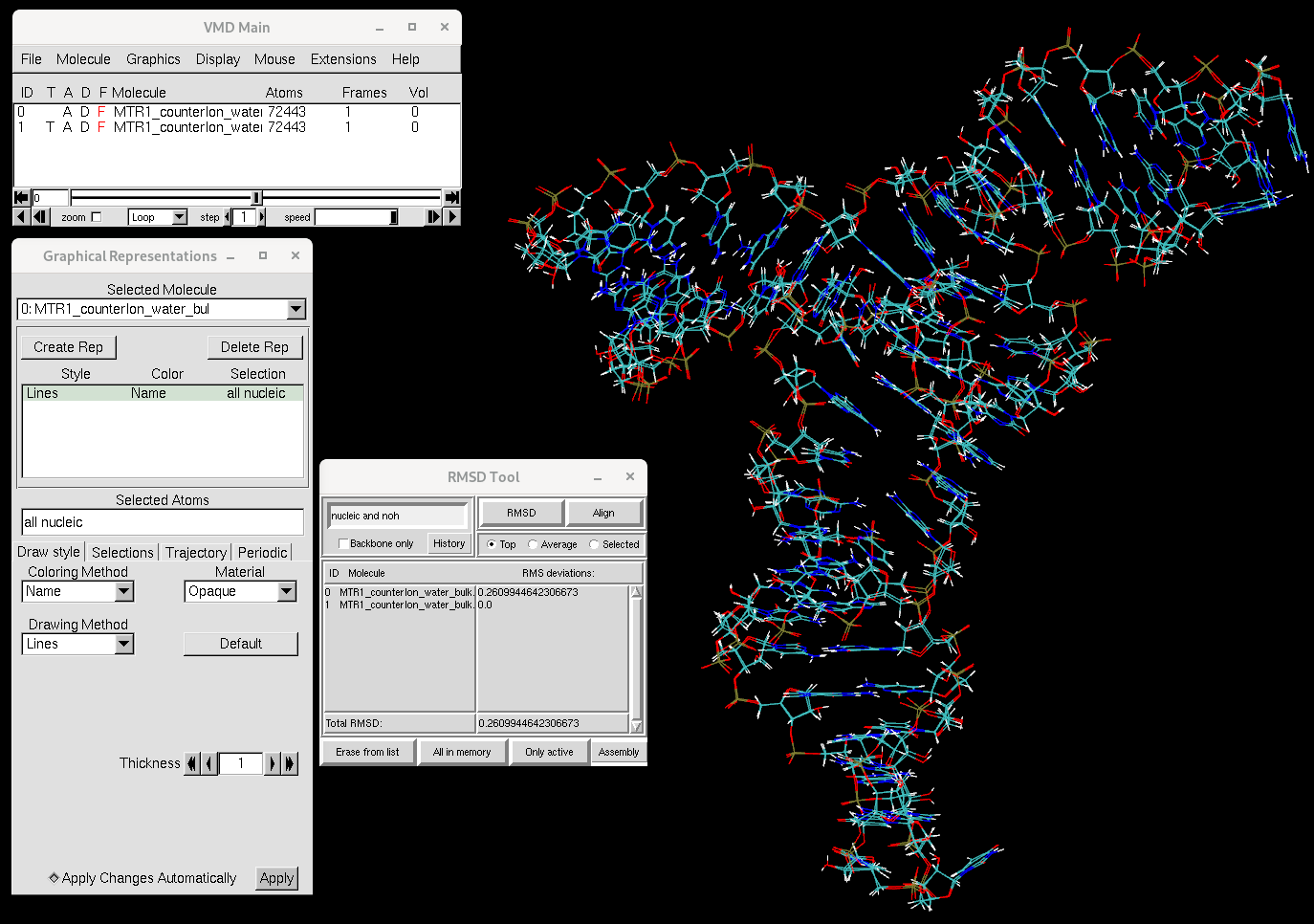
Figure 1. RMSD between the MTR1 structure before and after equilibration. RMSD is computed for RNA atoms.
You will see that the RNA structure has not changed much over the course of equilibration. Now let’s focus on the ions.
In the RMSD Calculator, change the selection from all nucleic to
ions.
Uncheck the Backbone only option if it is checked and compute the RMSD for the ions.
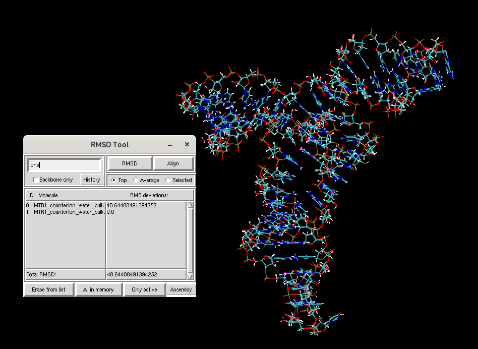
Figure 2. RMSD of ions in the MTR1 simulation box before and after equilibration.
You will see that the RMSD for the ions between the two structures is much larger than that of the RNA. To study the dynamics of the RNA, you will next learn to run production MD simulations starting from your equilibrated structure.
2.3.5. Running Production Simulations
In this section, you will run a very short 0.5 ns production molecular dynamics simulation without positional restraints on the RNA. In previous studies of this RNA system, production simulations converged on the order of tens of nanoseconds. Although longer time scales are desirable, such simulations cannot be performed within the time constraints of this workshop.
You have been provided the production MD input file:
This input file performs 0.5 ns of unrestrained dynamics in the isothermal–isobaric ensemble (NPT) and is intended to provide a brief introduction to running production simulations in AMBER.
You have also been provided the SLURM submission script used to run the production simulation:
2.3.5.1. The production SLURM script
The following SLURM script is used to run the production simulation. It takes as input the prefix of the AMBER topology and restart files and automatically increments the output file numbering.
#!/bin/bash
#SBATCH -o slurm-%j.out
#SBATCH -e slurm-%j.err
#SBATCH --nodes=1
#SBATCH --gpus=1
#SBATCH --ntasks-per-node=1
#SBATCH --partition=gpu-shared
#SBATCH -t 0-00:20:00
#SBATCH --no-requeue
#SBATCH --reservation=amber24gpu
#SBATCH --account=gue998

Base=${1}
Parm=${1}.parm7

mdin=mdins/11_Production_0.5ns.mdin

module load workshop/amber24/default

newname=""

if [[ $Base == *-run-* ]]; then
  prefix=${Base%-*}
  suffix=${Base##*-}
  if [[ $suffix =~ [0-9]+ ]]; then
    number=${suffix#*-}
    new_number=$(printf "%02d" $((number + 1)))
    newname="${prefix}-${new_number}"
  else
    newname="${Base}-01"
  fi
else
  newname="${Base}-01"
fi

exe=${AMBERHOME}/bin/pmemd.cuda_SPFP

$exe -O -p ${Parm} -c ${Base}.rst7 -i ${mdin} \
     -o ${newname}.mdout -inf ${newname}.mdinfo \
     -x ${newname}.nc -r ${newname}.rst7 -ref ${Base}.rst7
This script appends -01 to the input prefix when generating output
files. If the input prefix already contains a numeric suffix (e.g. when
restarting a simulation), the suffix is incremented to -02, -03,
and so on. This allows longer production simulations to be split into
multiple consecutive runs to accommodate HPC wall-time limits.
2.3.5.2. Preparing the production input files
Copy the equilibrated restart file and rename it for production:
cp 09_Equil_solute_Rwt2-run.rst7 MTR1_counterIon_water_bulk-run.rst7
Production MD will be run with a 4 fs timestep. To do this stably, hydrogen mass repartitioning (HMR) is applied. You have been provided the cpptraj input file used for this purpose:
The cpptraj input file used to apply hydrogen mass repartitioning is shown below:
parm MTR1_counterIon_water_bulk.parm7
hmassrepartition
parmwrite out MTR1_counterIon_water_bulk-run.parm7
go
quit
Run cpptraj to generate the HMR-modified topology file:
cpptraj -i hmr.in
This command generates MTR1_counterIon_water_bulk-run.parm7, which will be used for the production simulation.
2.3.5.3. Running the production simulation
Submit the production job:
sbatch prod.slurm MTR1_counterIon_water_bulk-run
The job should take approximately 10 minutes to complete. Output files
will be written with the prefix MTR1_counterIon_water_bulk-run-01.
2.3.5.4. Wrapping and visualization of the production trajectory
After the production simulation has completed, the resulting trajectory must be wrapped to account for periodic boundary conditions before visualization.
You have been provided a cpptraj input file for wrapping the production trajectory:
Wrap the structure:
cpptraj -i wrap_RNA_prod.in
This command produces the wrapped trajectory file centered.MTR1_counterIon_water_bulk-run-01.nc. This trajectory can now be visualized in VMD.
Open the trajectory in VMD:
vmd centered.MTR1_counterIon_water_bulk-run-01.nc \
    MTR1_counterIon_water_bulk-run.parm7
To use the same visualization representations as in the equilibration
section, you can source the VMD representation file provided for this
activity. (/path/Day1/HS2/Files/input/build/MTR_waterreps.txt)
Alternatively, you can load the trajectory and apply the representations directly from the command line:
vmd -e MTR_waterreps.txt \
    centered.MTR1_counterIon_water_bulk-run-01.nc \
    MTR1_counterIon_water_bulk-run.parm7
Inspect the dynamics of the different components. Below is a movie demonstration:
Warning
This was a very short production simulation. Realistically, it would be desirable to perform multiple independent long production simulations. In previous studies of MTR1, five independent production simulations of 150 ns each were performed. Analysis of the root mean square deviation (RMSD) indicated that the first 50 ns corresponded to equilibration, while the remaining 100 ns of each simulation were used for production analysis, resulting in a total of 500 ns of production data.
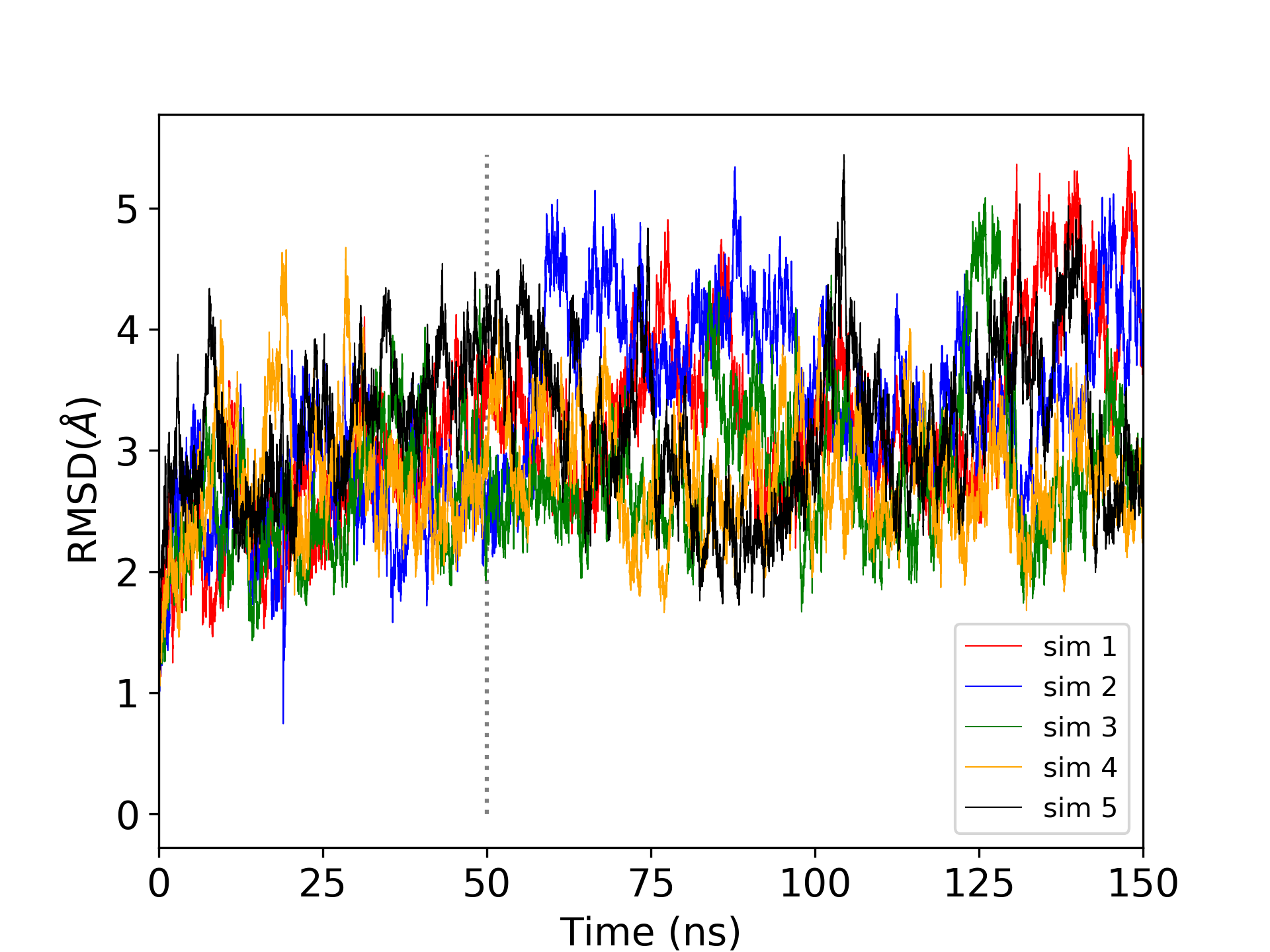
Figure 3. Root mean square deviation of the positions of heavy atoms with respect to the first trajectory frame over five independent 150 ns production simulations.
2.3.6. (Optional) Additional Exercise: Performing a brief energy minimization
The following exercise should only be performed if you have time left over
or are waiting for other simulations to run. In this exercise, you will
run the 000_Min step of the equilibration procedure independently.
You have already been introduced to the equilibration script
eqFromStratch.slurm. In this optional exercise, you will modify this
script to run only the initial minimization step on the CPU.
You have been provided the original equilibration SLURM script:
Copy the equilibration script and create a new script for the minimization only run:
[user@cluster] cp eqFromStratch.slurm eqFromStratch_000.slurm
Open eqFromStratch_000.slurm in a text editor (e.g. vim) and modify
the SLURM header so that the job runs on the CPU rather than on a GPU:
#!/bin/bash
#SBATCH -o slurm-%j.out
#SBATCH -e slurm-%j.err
#SBATCH --nodes=1
#SBATCH --ntasks-per-node=1
#SBATCH --partition=shared
#SBATCH --account=gue998
#SBATCH --reservation=amber24
#SBATCH -t 0-00:30:00
#SBATCH --no-requeue
Next, edit the script so that only the 000_Min step is executed. Delete
all other steps and retain only the following definition:
steps="\
000_Min \
"
In this case, only sander will be invoked, so no GPU resources are
required. The job is expected to finish in approximately 10 minutes.
Before submitting the job, verify that the Equil directory contains the
necessary files. If you are also running production simulations in the same
directory, that is fine. However, if you previously copied
000_Min-run.mdout from the reference output, you may need to delete it,
otherwise the script will detect that the step has already completed and
exit immediately.
The directory should contain the following:
[user@cluster] ls
MTR1_counterIon_water_bulk.parm7
MTR1_counterIon_water_bulk.rst7
eqFromStratch.slurm
eqFromStratch_000.slurm
mdins
restrnt.disang
Submit the job:
[user@cluster] sbatch eqFromStratch_000.slurm MTR1_counterIon_water_bulk
When the job is complete, monitor how the total energy (EAMBER)
decreases over the course of the minimization:
[user@cluster] grep -r EAMBER 000_Min-run.mdout | awk '{print $3}' | head -n10 > ene.dat
Plot the energy using xmgrace. Make sure the appropriate modules are
loaded first. It may be more convenient to run xmgrace in a separate
terminal:
[user@cluster] xmgrace ene.dat
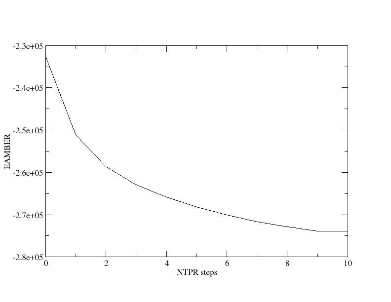
Figure 4. Total energy output every 50 optimization steps during
the 000_Min minimization.
You will observe that the total energy (in kcal/mol) decreases rapidly at the beginning of the minimization and then begins to plateau. In this run, the energy was printed every 50 minimization steps.
Open 000_Min-run.mdout in a text editor and inspect the individual energy components:
  NSTEP       ENERGY          RMS            GMAX         NAME    NUMBER
     1       1.7197E+06     6.7827E+04     2.2501E+07     N3       1730

BOND    =     5038.2053  ANGLE   =      397.2193  DIHED      =     1511.0059
VDWAALS =  1926187.1298  EEL     =  -206390.2786  HBOND      =        0.0000
1-4 VDW =      697.4115  1-4 EEL =    -7778.5268  RESTRAINT  =        0.0000


  NSTEP       ENERGY          RMS            GMAX         NAME    NUMBER
    50      -2.3201E+05     4.6787E+00     6.6797E+02     C6       1723

BOND    =    22954.6607  ANGLE   =      746.4316  DIHED      =     1649.0907
VDWAALS =    27936.2925  EEL     =  -278521.9124  HBOND      =        0.0000
1-4 VDW =      650.9327  1-4 EEL =    -7954.8135  RESTRAINT  =      533.4714
EAMBER  =  -232539.3177
You will notice that the van der Waals energy decreases rapidly at the beginning of the minimization as bad contacts are relieved. This illustrates the importance of a gradual and well-controlled equilibration procedure.