Hands-On Session 10: Perform AFE simulations for Absolute Binding, using free energy workflows

Zeke A. Piskulich¹, Patricio Barletta¹, Ryan Snyder¹, Harsh Amin¹, and Darrin M. York¹

¹Laboratory for Biomolecular Simulation Research, Institute for Quantitative Biomedicine and Department of Chemistry and Chemical Biology, Rutgers University, Piscataway, NJ 08854, USA

Learning objectives

Learn how to build simulation boxes for absolute binding free energy calculations (ABFE) using AmberTools
Understand the options for solvating simulation boxes and adding ions
Learn how to make consistent solvent boxes for both the bound and unbound states of the ligand.

Learn how to equilibrate the endstates in preparation for running absolute binding free energy calculations (ABFE).

Learn how to determine Boresch restraints from end-state trajectories.

Learn how to set up and generate lambda windows for absolute binding free energy (ABFE) calculations starting from an equilbrated end-state.
Learn how to run ABFE calculations using Amber

Learn how to analyze absolute binding free energy calculations using FE-Toolkit and Edgembar.
Understand how to interpret the results of ABFE calculations for the Tyk2 system.

Activities

        flowchart LR
Download["Download activity files<br>Inputs - build_files.tar.gz<br>Outputs - extracted build_files"]


 subgraph Aqueous_Leg ["Aqueous Phase"]
   direction TB
   AL1["Load ligand files and leaprc<br>Inputs - binder_XXX.lib binder_XXX.frcmod binder_XXX.pdb"]
   AL2["Build prebox with tleap<br>Commands - setbox centers<br>addions2 Na+ 0 Cl- 0<br>solvateoct TIP4PBOX 16.0<br>Outputs - prebox_binder_XXX.parm7 .rst7"]
   AL3["Count waters and compute ions<br>Subprogram - count_waters.py<br>Calc - N_ions = N_water * 0.150 / 55<br>Outputs - N ions per type"]
   AL4["Add ions and save final binder<br>Command - addionsrand mol Na+ 7 Cl- 7 6.0 (example)<br>Outputs - binder_XXX.parm7 .rst7"]
 end

 subgraph Complex_Leg ["Bound Complex"]
   direction TB
   CL1["Load ligand and protein files and leaprc<br>Inputs - binder_XXX.lib binder_XXX.frcmod binder_XXX.pdb target.pdb"]
   CL2["Combine and build prebox with tleap<br>Commands - combine mol prot<br>setbox centers<br>solvateoct TIP4PBOX 14.0<br>Outputs - prebox_target_XXX.parm7 .rst7"]
   CL3["Count waters and compute ions for complex<br>Subprogram - count_waters.py<br>Example - 11023 waters -> 30 Na+ 30 Cl-<br>Outputs - N ions per type"]
   CL4["Add ions to complex and save final system<br>Command - addionsrand complex Na+ 30 Cl- 30 6.0 (example)<br>Outputs - target_XXX.parm7 .rst7"]
 end

 %% Parallel legs from the common Download node
 Download --> AL1
 Download --> CL1

 AL1 --> AL2
 CL1 --> CL2

 AL2 --> AL3
 CL2 --> CL3

 AL3 --> AL4
 CL3 --> CL4

 %% Join the two legs into the optional HMR step
 AL4 --> HMR["Optional Hydrogen Mass Repartitioning<br>Tool - ParmEd<br>Commands - parm file<br>hmassrepartition<br>outparm *_hmr.parm7<br>Outputs - *_hmr.parm7"]
 CL4 --> HMR

 HMR --> END["Ready for minimization equilibration and ABFE workflows<br>Notes - repeat for each ligand; keep solvent box consistency if desired"]

Determining Boresch Restraints

For this activity, we will be starting from the equilibrated end-state trajectory of a Tyk2-ligand complex in its bound state. These files were generated in the activity Equilibrating Endstates in ABFE Calculations (Tyk2); however, for convenience we have provided the necessary files below to get you started.

Attention

Update the download link to point to the finalized activity files once they are uploaded.

Boresch restraints are a type of positional restraint used in molecular dynamics simulations to maintain the relative position and orientation of a ligand within a binding site. They are particularly useful in absolute binding free energy calculations, where it is essential to keep the ligand in place while decoupling its interactions with the environment.

The Boresch restraint method involves defining a set of six restraints based on three atoms from the ligand and three atoms from the protein. These restraints include:

One distance Restraint
Two Angle Restraints
Three Dihedral Restraints

These restraints work together to fix the ligand’s position and orientation relative to the protein, allowing for accurate free energy calculations.

Note

This theory section should be expanded with a more detailed explanation of the mathematical formulation of Boresch restraints, including equations and diagrams to illustrate the concepts.

Note

Much of the below theoretical discussion comes from Boresch et al., J. Phys. Chem. B, 2003, 107 (35), pp 9535–9551. DOI: 10.1021/jp0217839.

The goal of Boresch restraints is to define a known set of lambda-dependent restraints that can be applied to the ligand in the bound state to keep it in place while decoupling its interactions with the environment, while also allowing for an analytical correction to the free energy to account for the restraints.

Roughly, the situation that needs to be corrected for is:

\[(P \cdot L)_{H_2O} \rightarrow^{\Delta A_r} (P)_{H_2O} + (L)_{H_2O},\]

Where here, (P cdot L)_{H_2O} is the protein-ligand complex in water with restraints applied, (P)_{H_2O} is the protein in water, and (L)_{H_2O} is the ligand in water. \(\Delta A_r\) is the free energy change associated with removing the restraints from the complex in water.

Because the ligand is in the dummy state when decoupled, the ligand does not have interactions with the protein or solvent and thus the restraints are the only interactions with external sources it feels. The potential energy function for the system is:

\[U = U_P(r_P) + U_L(r_L) + U_{r}(r_P, r_L).\]

Here, there are terms coming from the protein (\(U_P\)), the ligand (\(U_L\)), and the restraints (\(U_r\)).

The contribution to the free energy that comes from the restraints can be written as:

\[\Delta A_r = -k_B T \ln \left( \frac{Z_P Z_L}{Z_{P \cdot L}} \right)\]

Where \(Z_{P \cdot L}\) is the partition function of the restrained complex, \(Z_P\) is the partition function of the protein, and \(Z_L\) is the partition function of the ligand.

This calculation is feasible analytically when the restraints are chosen such that

\[Z_{P \cdot L} = Z_P \times Z_L \times Z_r,\]

or in other words, choosing the restraints such that the partition function can be factored into independent contributions from the protein, ligand, and restraints.

After a few assumptions (Rigid Rotor) the final expression for the partition function is given by:

\[Z_{P \cdot L} = r^2_{aA,0} \sin(\theta_{A,0}) \frac{(2 \pi k_B T)^3}{\sqrt{K_r K_{\theta^A} K_{\theta^B} K_{\phi^A} K_{\phi^B} K_{\phi^C}}},\]

Finally, the free energy contribution from the restraints can be expressed as:

\[\Delta A_r = -k_B T \ln \left[\frac{8\pi^2V\sqrt{K_rK_{\theta^A}K_{\theta^B}K_{\phi^A}K_{\phi^B}K_{\phi^C}}}{r^2_{aA,0} \sin(\theta_{A,0}) \sin(\theta_{B,0}) (2\pi k_B T)^3} \right]\]

Where \(r_{aA,0}\) and \(\theta_{A,0}\) are the equilibrium distance and angle values for the restraints, and \(K_r\), \(K_{\theta^A}\), \(K_{\theta^B}\), \(K_{\phi^A}\), \(K_{\phi^B}\), and \(K_{\phi^C}\) are the force constants for the respective restraints.

How to Determine Boresch Restraints

To determine the Boresch restraints for your system, you will need to analyze an equilibrated trajectory for the protein-ligand complex.

Note

If you have been following along with the Tyk2 ABFE Activities, it is very likely that you have already generated a trajectory. It very likely that your trajectory will be different from the one included here, but the steps to generate the boresch restraints will be the same. Don’t be surprised if your final results differ from those presented here!

For this activity, we will be using the following python code, which you should save as generate_boresch_restraints.py:

#!/usr/bin/env python3
"""Generate Boresch restraints from equilibration trajectory.

This script scans ligand heavy atoms and nearby protein heavy atoms to
identify stable anchor pairs, computes Boresch degrees of freedom over
the trajectory, and prints/writes restraint parameters.

Behavior is preserved from the original script but reorganized for
readability and reuse.
"""

import argparse
import logging
from pathlib import Path

import MDAnalysis as mda
from MDAnalysis.analysis.distances import dist
from MDAnalysis.lib.distances import calc_dihedrals
import numpy as np
from numpy.linalg import norm
import matplotlib.pyplot as plt


LOG = logging.getLogger(__name__)


def parse_args():
    """Parse command-line arguments.

    Returns
    -------
    argparse.Namespace
        Object with attributes:
        - topology: str, path to topology file (default './unisc.parm7')
        - trajectory: str, path to trajectory file (default 'equil1/real_eq.nc')
        - ligand_sel: str, MDAnalysis selection string for ligand heavy atoms
        - cutoff: float, distance in angstroms to search for nearby protein atoms
        - num_pairs: int, number of lowest-standard-deviation pairs to show/select
        - max_pairs_traj: int, maximum number of pairs to analyze over the trajectory
        - out_rest: str, output filename to write AMBER restraint input
        - fig_prefix: str, prefix for any figures written

    Notes
    -----
    This function only constructs and returns the parsed arguments object.
    Documentation in tutorials should show running the script like:

    $ python generate_boresch_restraints.py --topology my.parm7 --trajectory my.nc
    """
    p = argparse.ArgumentParser(
        description="Generate Boresch restraints from equilibration trajectory"
    )
    p.add_argument("--topology", type=str, default="./unisc.parm7", help="Topology file")
    p.add_argument("--trajectory", type=str, default="equil1/real_eq.nc", help="Equilibration trajectory file")
    p.add_argument("--ligand-sel", type=str, default="resid 1 and not name H*", help="Selection for ligand heavy atoms")
    p.add_argument("--cutoff", type=float, default=10.0, help="Cutoff (angstrom) to search nearby protein atoms")
    p.add_argument("--num-pairs", type=int, default=5, help="Number of low-SD pairs to show/select")
    p.add_argument("--max-pairs-traj", type=int, default=200, help="Max pairs to analyze over trajectory")
    p.add_argument("--out-rest", type=str, default="rest.in", help="Output restraint file")
    p.add_argument("--fig-prefix", type=str, default="boresch", help="Prefix for saved figures")
    return p.parse_args()


def find_anchor_pairs(u, ligand_sel="resid 1 and not name H*", cutoff=10.0):
    """Find candidate ligand-protein anchor atom pairs.

    Parameters
    ----------
    u : MDAnalysis.Universe
        Loaded universe containing topology and trajectory.
    ligand_sel : str
        MDAnalysis selection string identifying ligand heavy atoms (no H).
    cutoff : float
        Distance cutoff (in Å) used to find protein heavy atoms near each
        ligand heavy atom.

    Returns
    -------
    dict
        Mapping (ligand_atom_index, protein_atom_index) -> dict with key
        'dists' initialized to an empty list. Distances over the trajectory
        will be appended to this list by :func:`collect_distances`.

    Behavior details
    ----------------
    - Protein atoms are selected with the MDAnalysis "around" syntax.
    - The returned atom indices are MDAnalysis global atom indices (0-based).
    """
    lig_heavy = u.select_atoms(ligand_sel)
    anchors = {}
    for lig_atom in lig_heavy:
        # select protein heavy atoms within cutoff of ligand atom
        prot_sel = f"(protein or resname PRT) and (around {cutoff} index {lig_atom.index}) and (not name H*)"
        prot_atoms = u.select_atoms(prot_sel)
        for prot_atom in prot_atoms:
            anchors[(lig_atom.index, prot_atom.index)] = {"dists": []}
    return anchors


def collect_distances(u, anchors):
    """Populate `anchors` with distance time series from the trajectory.

    Parameters
    ----------
    u : MDAnalysis.Universe
        Universe that has already been loaded with topology and trajectory.
    anchors : dict
        Dictionary produced by :func:`find_anchor_pairs`. Keys are (lig_idx, prot_idx).

    Returns
    -------
    dict
        The same anchors dict with 'dists' converted to numpy arrays and
        augmented with 'avg_dist' and 'sd_dist' for each pair.

    Notes
    -----
    - Distances are computed frame-by-frame using MDAnalysis distance routines
      with periodic box handling (box=frame.dimensions).
    - For performance, this function iterates over frames and pairs; for large
      trajectories or many pairs consider vectorized approaches or sampling.
    """
    # Iterate trajectory and collect distances for each pair
    for frame in u.trajectory:
        for lig_idx, prot_idx in list(anchors.keys()):
            # compute distance using MDAnalysis distance routine
            distance = dist(
                mda.AtomGroup([u.atoms[lig_idx]]),
                mda.AtomGroup([u.atoms[prot_idx]]),
                box=frame.dimensions,
            )[2][0]
            anchors[(lig_idx, prot_idx)]["dists"].append(distance)

    # convert lists to numpy arrays and compute stats
    for pair in anchors.keys():
        anchors[pair]["dists"] = np.array(anchors[pair]["dists"])
        anchors[pair]["avg_dist"] = anchors[pair]["dists"].mean()
        anchors[pair]["sd_dist"] = anchors[pair]["dists"].std()

    return anchors


def report_low_sd_pairs(u, anchors, n=5):
    """Report and return the top-N anchor pairs with lowest distance SD.

    Parameters
    ----------
    u : MDAnalysis.Universe
        Universe used only for pretty-printing atom information.
    anchors : dict
        Anchors dict returned by :func:`collect_distances`.
    n : int
        Number of pairs to report.

    Returns
    -------
    list
        Ordered list of (lig_idx, prot_idx) tuples sorted by ascending SD.

    This function logs informative lines that can be included in a tutorial
    to show how candidate anchor pairs are selected based on stability.
    """
    ordered = [item[0] for item in sorted(anchors.items(), key=lambda it: it[1]["sd_dist"]) ]
    LOG.info("Top %d pairs by lowest SD:", n)
    for i, pair in enumerate(ordered[:n]):
        a, b = pair
        LOG.info("Pair %d: %s - avg %.2f SD %.2f", i + 1, (u.atoms[a], u.atoms[b]), anchors[pair]["avg_dist"], anchors[pair]["sd_dist"])
    return ordered


def get_anchor_ats(a1_idx, u):
    """Select three anchor atoms around a given atom index.

    Parameters
    ----------
    a1_idx : int
        Index of the primary anchor atom (0-based, MDAnalysis indexing).
    u : MDAnalysis.Universe
        Universe containing topology information - used to query bonded atoms.

    Returns
    -------
    tuple
        (a1_idx, a2_idx, a3_idx) where a2 and a3 are heavy atoms chosen to be
        bonded neighbors of a1 (or the next atoms along the chain if at a terminus).

    Behavior and edge cases
    -----------------------
    - The function prefers bonded heavy atoms that are not hydrogens.
    - If a1 is terminal (only a single heavy neighbor), the function walks
      one more bond along that neighbor to find a3.
    - If no bonded heavy atoms are found an exception is raised; calling
      code should ensure anchor candidates are sensible (heavy atoms typically have bonded neighbors).

    Rationale
    ---------
    These three anchor atoms are used to define internal angles/dihedrals
    in Boresch-style restraints: the ligand anchor (a1,a2,a3) will be paired
    with a receptor anchor triplet to define distance/angle/dihedral restraints.
    """
    a1_at = u.atoms[a1_idx]
    # select bonded heavy atoms (not hydrogens)
    bonded_heavy = a1_at.bonded_atoms.select_atoms("not name H*")
    if len(bonded_heavy) == 0:
        raise RuntimeError(f"No bonded heavy atoms found for atom index {a1_idx}")

    a2_idx = bonded_heavy[0].index
    if len(bonded_heavy) > 1:
        a3_idx = bonded_heavy[1].index
    else:
        # step one further away along heavy atoms
        next_heavy = bonded_heavy[0].bonded_atoms.select_atoms("not name H*")
        # prefer the second atom if that avoids going back to a1_idx
        a3_candidate = next_heavy[1].index if len(next_heavy) > 1 else next_heavy[0].index
        if a3_candidate == a1_idx and len(next_heavy) > 1:
            a3_candidate = next_heavy[0].index
        a3_idx = a3_candidate

    return a1_idx, a2_idx, a3_idx


# Geometry helpers
def get_distance(idx1, idx2, u):
    """Compute Euclidean distance (Å) between two atoms by index.

    Parameters
    ----------
    idx1, idx2 : int
        Atom indices (0-based).
    u : MDAnalysis.Universe

    Returns
    -------
    float
        Distance in Å.
    """
    return dist(mda.AtomGroup([u.atoms[idx1]]), mda.AtomGroup([u.atoms[idx2]]), box=u.dimensions)[2][0]


def get_angle(idx1, idx2, idx3, u):
    """Compute angle (radians) defined by three atoms A-B-C.

    Parameters
    ----------
    idx1 : int
        Index of atom C (first argument in original function definition)
    idx2 : int
        Index of atom B (central atom)
    idx3 : int
        Index of atom A (last argument)
    u : MDAnalysis.Universe

    Returns
    -------
    float
        Angle in radians.

    Notes
    -----
    The ordering follows the original script: get_angle(idx1, idx2, idx3)
    returns the angle at atom idx2 formed by vectors (A-B) and (C-B) where
    A = idx3, B = idx2, C = idx1.
    """
    C = u.atoms[idx1].position
    B = u.atoms[idx2].position
    A = u.atoms[idx3].position
    BA = A - B
    BC = C - B
    angle = np.arccos(np.dot(BA, BC) / (norm(BA) * norm(BC)))
    return angle


def get_dihedral(idx1, idx2, idx3, idx4, u):
    """Compute dihedral (torsion) angle in radians for four atoms.

    Parameters
    ----------
    idx1, idx2, idx3, idx4 : int
        Atom indices specifying the torsion in the order used by MDAnalysis.
    u : MDAnalysis.Universe

    Returns
    -------
    float
        Dihedral angle in radians (range -pi..pi).

    Notes
    -----
    MDAnalysis' calc_dihedrals returns values in the range (-pi, pi].
    """
    positions = [u.atoms[idx].position for idx in [idx1, idx2, idx3, idx4]]
    dihedral = calc_dihedrals(positions[0], positions[1], positions[2], positions[3], box=u.dimensions)
    return dihedral


def get_boresch_dof(l1, l2, l3, r1, r2, r3, u):
    """Compute the Boresch degrees of freedom for a given anchor sextet.

    Parameters
    ----------
    l1,l2,l3 : int
        Indices of the three ligand anchor atoms (l1 is bonded to receptor r1).
    r1,r2,r3 : int
        Indices of the three receptor anchor atoms (r1 bonded to ligand l1).
    u : MDAnalysis.Universe

    Returns
    -------
    tuple
        (r, thetaA, thetaB, phiA, phiB, phiC, thetaR, thetaL)

    Where
    -----
    - r : float, distance between r1 and l1 (Å)
    - thetaA, thetaB : floats, angles (radians)
    - phiA, phiB, phiC : floats, dihedrals (radians)
    - thetaR, thetaL : internal receptor/ligand angles (radians)

    Usage
    -----
    These values correspond to the common variables used to define a set
    of Boresch restraints (one distance, two angles, three dihedrals).
    """
    # Ordering r3,r2,r1,l1,l2,l3 as in original
    r = get_distance(r1, l1, u)
    thetaA = get_angle(r2, r1, l1, u)
    thetaB = get_angle(r1, l1, l2, u)
    phiA = get_dihedral(r3, r2, r1, l1, u)
    phiB = get_dihedral(r2, r1, l1, l2, u)
    phiC = get_dihedral(r1, l1, l2, l3, u)
    thetaR = get_angle(r3, r2, r1, u)
    thetaL = get_angle(l1, l2, l3, u)
    return r, thetaA, thetaB, phiA, phiB, phiC, thetaR, thetaL


def analyze_boresch_over_traj(u, pairs, max_pairs=200):
    """Compute time series and statistics for Boresch DOF across trajectory.

    Parameters
    ----------
    u : MDAnalysis.Universe
        Universe with trajectory.
    pairs : iterable
        Iterable of (l1_idx, r1_idx) anchor pairs to analyze.
    max_pairs : int
        Maximum number of pairs to process (for performance control).

    Returns
    -------
    dict
        Mapping pair -> dict with keys:
        - 'anchor_ats': [l1,l2,l3,r1,r2,r3]
        - for each dof e.g. 'r', 'phiA', etc.: dict with 'values' (np.array), 'avg', 'sd', 'k'
        - 'tot_var': sum of variances used to rank pair suitability

    Important details
    -----------------
    - For dihedral DOFs (phiA/B/C) this function applies a circular-statistics
      aware procedure to compute mean and standard deviation so that periodicity
      is correctly handled (angles near -pi and +pi are treated continuously).
    - Force constants k are estimated assuming a Gaussian distribution via
      k = RT / sd^2, where RT is approximated as 0.593 kcal/mol at 289 K in
      the original script. This is the same convention and will be halved
      later when writing restraint parameters to be consistent with external tools.
    """
    boresch = {}
    boresch_dof_list = ["r", "thetaA", "thetaB", "phiA", "phiB", "phiC", "thetaR", "thetaL"]

    for pair in pairs[:max_pairs]:
        boresch[pair] = {}
        l1_idx, r1_idx = pair
        _, l2_idx, l3_idx = get_anchor_ats(l1_idx, u)
        _, r2_idx, r3_idx = get_anchor_ats(r1_idx, u)
        boresch[pair]["anchor_ats"] = [l1_idx, l2_idx, l3_idx, r1_idx, r2_idx, r3_idx]

        for dof in boresch_dof_list:
            boresch[pair][dof] = {"values": []}

        n_frames = len(u.trajectory)
        for i, frame in enumerate(u.trajectory):
            r, thetaA, thetaB, phiA, phiB, phiC, thetaR, thetaL = get_boresch_dof(
                l1_idx, l2_idx, l3_idx, r1_idx, r2_idx, r3_idx, u
            )
            boresch[pair]["r"]["values"].append(r)
            boresch[pair]["thetaA"]["values"].append(thetaA)
            boresch[pair]["thetaB"]["values"].append(thetaB)
            boresch[pair]["phiA"]["values"].append(phiA)
            boresch[pair]["phiB"]["values"].append(phiB)
            boresch[pair]["phiC"]["values"].append(phiC)
            boresch[pair]["thetaR"]["values"].append(thetaR)
            boresch[pair]["thetaL"]["values"].append(thetaL)

        # After frames loop compute statistics
        boresch[pair]["tot_var"] = 0.0
        for dof in boresch_dof_list:
            values = np.array(boresch[pair][dof]["values"])
            boresch[pair][dof]["values"] = values
            avg = values.mean()
            boresch[pair][dof]["avg"] = avg

            if dof.startswith("phi"):
                # circular statistics handling for dihedrals
                corrected_vals = []
                for val in values:
                    dtheta = abs(val - avg)
                    corrected_vals.append(min(dtheta, 2 * np.pi - dtheta))
                corrected_vals = np.array(corrected_vals)
                boresch[pair][dof]["sd"] = corrected_vals.std()

                # correct mean
                periodic_bound = avg - np.pi
                if periodic_bound < -np.pi:
                    periodic_bound += 2 * np.pi
                corrected_avg_vals = [v + 2 * np.pi if v < periodic_bound else v for v in values]
                m_corr = np.array(corrected_avg_vals).mean()
                if m_corr > np.pi:
                    boresch[pair][dof]["avg"] = m_corr - 2 * np.pi
                else:
                    boresch[pair][dof]["avg"] = m_corr
            else:
                boresch[pair][dof]["sd"] = values.std()

            if dof not in ("thetaR", "thetaL"):
                boresch[pair]["tot_var"] += boresch[pair][dof]["sd"] ** 2

            boresch[pair][dof]["k"] = 0.593 / (boresch[pair][dof]["sd"] ** 2)

    return boresch


def select_pairs(boresch_dict):
    """Select suitable anchor pairs based on geometric filters.

    Parameters
    ----------
    boresch_dict : dict
        Output from :func:`analyze_boresch_over_traj`.

    Returns
    -------
    list
        Filtered list of pairs, ordered by increasing tot_var.

    Filtering criteria
    ------------------
    - Distance r average must be > 1.0 Å (filters out extremely close/invalid pairs)
    - Average angles thetaA and thetaB must be within (0.52, 2.62) radians (~30°-150°)

    These thresholds were chosen empirically to avoid degenerate restraints.
    """
    # order by tot_var
    ordered = [item[0] for item in sorted(boresch_dict.items(), key=lambda it: it[1]["tot_var"]) ]
    # filter by distance and internal angles
    selected = []
    for pair in ordered:
        cond_dist = boresch_dict[pair]["r"]["avg"] > 1.0
        avg_angles = [boresch_dict[pair][a]["avg"] for a in ("thetaA", "thetaB")]
        cond_angles = all((0.52 < ang < 2.62) for ang in avg_angles)
        if cond_dist and cond_angles:
            selected.append(pair)
    return selected


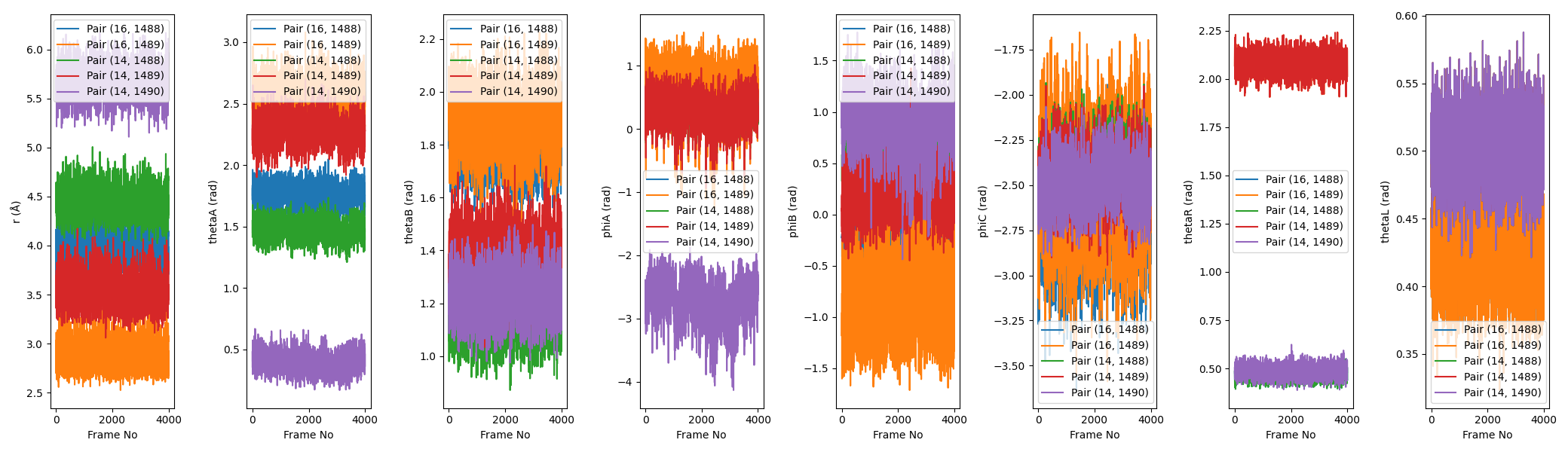
def plot_time_series(boresch_dict, pairs, fig_prefix="boresch", num_pairs=5):
    """Plot time series for each Boresch DOF for the top candidate pairs.

    The plotting function will unwrap phi (dihedral) time series around the
    computed circular mean so that the plot does not show large jumps at the
    -π/π periodic boundary. Figures are saved with the prefix provided.

    Parameters
    ----------
    boresch_dict : dict
        Boresch results as produced by :func:`analyze_boresch_over_traj`.
    pairs : list
        Candidate pairs (ordering is preserved); only the first `num_pairs`
        are plotted.
    fig_prefix : str
        Prefix used for saved figure filenames.
    num_pairs : int
        Number of pairs to include in the plot (default 5).
    """
    dofs = ["r", "thetaA", "thetaB", "phiA", "phiB", "phiC", "thetaR", "thetaL"]
    n_dof = len(dofs)
    fig, axs = plt.subplots(1, n_dof, figsize=(2.6 * n_dof, 6))

    def _unwrap_to_mean(values, mean):
        """Shift angular values by multiples of 2*pi so they lie within (mean-pi, mean+pi]."""
        return mean + ((values - mean + np.pi) % (2 * np.pi) - np.pi)

    for i, dof in enumerate(dofs):
        for j, pair in enumerate(list(boresch_dict.keys())[:num_pairs]):
            vals = boresch_dict[pair][dof]["values"]
            # For dihedrals (phi) unwrap values around their mean to avoid jumps at the -pi/pi boundary
            if dof.startswith("phi"):
                mean = boresch_dict[pair][dof].get("avg", 0.0)
                vals_plot = _unwrap_to_mean(vals, mean)
            else:
                vals_plot = vals

            axs[i].plot(np.arange(len(vals_plot)), vals_plot, label=f"Pair {pair}")

        axs[i].set_xlabel("Frame No")
        axs[i].set_ylabel("r (\u212B)" if dof == "r" else f"{dof} (rad)")
        axs[i].legend()
    fig.tight_layout()
    fig_file = f"{fig_prefix}_timeseries.png"
    fig.savefig(fig_file)
    LOG.info("Saved time series figure to %s", fig_file)


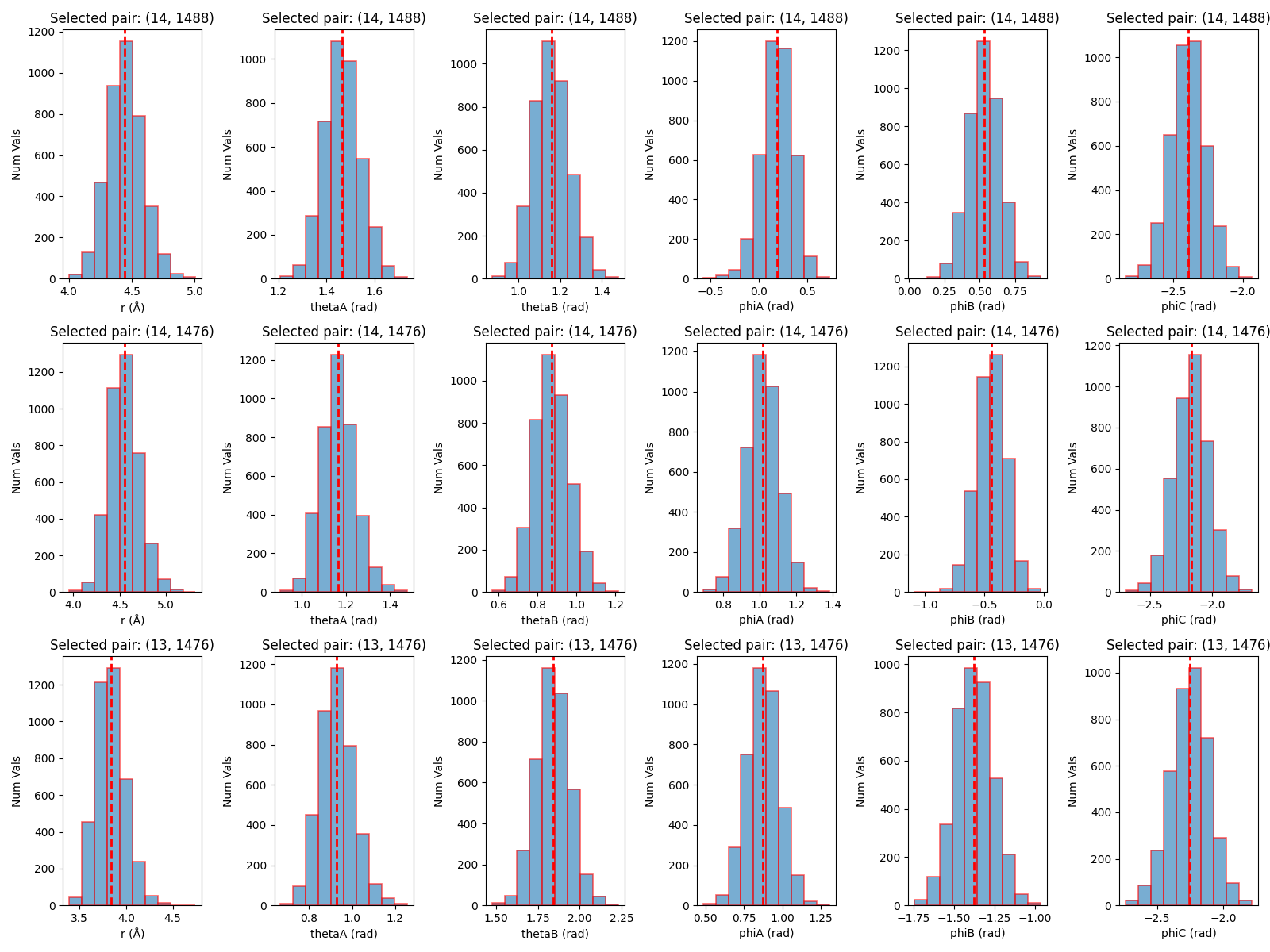
def plot_histograms(boresch_dict, pairs, fig_prefix="boresch", highlight_pairs=None):
    """Plot histograms of DOF distributions for top candidate pairs.

    Parameters
    ----------
    boresch_dict : dict
        Boresch data structure.
    pairs : list
        Candidate pairs selected for plotting.
    fig_prefix : str
        Prefix for saved histogram images.

    Notes
    -----
    - Histograms include a vertical dashed line showing the computed average.
    - Dihedral values are plotted in their stored range (after circular
      averaging), which avoids misleading binning across the -π/π boundary.
    """
    chosen = pairs[:3]
    dof_order = ["r", "thetaA", "thetaB", "phiA", "phiB", "phiC"]
    fig, axs = plt.subplots(len(chosen), len(dof_order), figsize=(16, 4 * len(chosen)))
    for pi, pair in enumerate(chosen):
        for di, dof in enumerate(dof_order):
            ax = axs[pi][di] if len(chosen) > 1 else axs[di]
            vals = boresch_dict[pair][dof]["values"]
            # draw histogram and get patch artists so we can outline selected pairs
            n, bins, patches = ax.hist(vals, bins=10)
            ax.axvline(x=boresch_dict[pair][dof]["avg"], color="r", linestyle="dashed", linewidth=2)
            # If this pair is in the highlight set, outline the bars and add title
            if highlight_pairs and pair in highlight_pairs:
                for p in patches:
                    p.set_edgecolor('red')
                    p.set_linewidth(1.2)
                    p.set_alpha(0.6)
                ax.set_title(f"Selected pair: {pair}")
            ax.set_xlabel("r (\u212B)" if dof == "r" else f"{dof} (rad)")
            ax.set_ylabel("Num Vals")
    fig.tight_layout()
    fig_file = f"{fig_prefix}_histograms.png"
    fig.savefig(fig_file)
    LOG.info("Saved histogram figure to %s", fig_file)


def print_boresch_params(pair, boresch_dict, out_rest="rest.in"):
    """Write out restraint parameters for a chosen anchor pair.

    Parameters
    ----------
    pair : tuple
        Anchor pair tuple returned by selection routines.
    boresch_dict : dict
        Results structure from :func:`analyze_boresch_over_traj`.
    out_rest : str
        Output filename for the AMBER restraint file (default 'rest.in').

    Behavior
    --------
    - Prints a JSON-like single-line summary to stdout suitable for parsing
      by tutorial readers or downstream tools.
    - Writes an AMBER &rst formatted restraint file where atom indices are
      converted to AMBER's 1-based indexing.
    - Force constants are halved in the output to match the energy definition
      used by some external MD codes (consistent with the original script).
    """
    l1, l2, l3, r1, r2, r3 = boresch_dict[pair]["anchor_ats"]
    r0 = boresch_dict[pair]["r"]["avg"]
    thetaA0 = boresch_dict[pair]["thetaA"]["avg"]
    thetaB0 = boresch_dict[pair]["thetaB"]["avg"]
    phiA0 = boresch_dict[pair]["phiA"]["avg"]
    phiB0 = boresch_dict[pair]["phiB"]["avg"]
    phiC0 = boresch_dict[pair]["phiC"]["avg"]
    kr = boresch_dict[pair]["r"]["k"] / 2
    kthetaA = boresch_dict[pair]["thetaA"]["k"] / 2
    kthetaB = boresch_dict[pair]["thetaB"]["k"] / 2
    kphiA = boresch_dict[pair]["phiA"]["k"] / 2
    kphiB = boresch_dict[pair]["phiB"]["k"] / 2
    kphiC = boresch_dict[pair]["phiC"]["k"] / 2

    json_str = (
        '{"anchor_points":{"r1":%d, "r2":%d, "r3":%d, "l1":%d, "l2":%d, "l3":%d},'
        '"equilibrium_values":{"r0":%.2f, "thetaA0":%.2f, "thetaB0":%.2f, "phiA0":%.2f, "phiB0":%.2f, "phiC0":%.2f},'
        '"force_constants":{"kr":%.2f, "kthetaA":%.2f, "kthetaB":%.2f, "kphiA":%.2f, "kphiB":%.2f, "kphiC":%.2f}}'
    ) % (r1, r2, r3, l1, l2, l3, r0, thetaA0, thetaB0, phiA0, phiB0, phiC0, kr, kthetaA, kthetaB, kphiA, kphiB, kphiC)

    print(json_str)

    # write AMBER restraint input (indices are 1-based in AMBER)
    with open(out_rest, "w") as fh:
        fh.write(f"&rst iat={r1+1},{l1+1},0\n")
        fh.write(f"  r1={0.0:.5f},r2={r0:.5f},r3={r0:.5f},r4=999.000,rk2={kr:.2f}, rk3={kr:.2f}/\n")
        fh.write(f"&rst iat={r2+1},{r1+1},{l1+1},0\n")
        fh.write(f"  r1={-180.0:.5f},r2={np.degrees(thetaA0):.5f},r3={np.degrees(thetaA0):.5f},r4=180.000,rk2={kthetaA:.2f}, rk3={kthetaA:.2f}/\n")
        fh.write(f"&rst iat={r1+1},{l1+1},{l2+1},0\n")
        fh.write(f"  r1={-180.0:.5f},r2={np.degrees(thetaB0):.5f},r3={np.degrees(thetaB0):.5f},r4=180.000,rk2={kthetaB:.2f}, rk3={kthetaB:.2f}/\n")
        fh.write(f"&rst iat={r3+1},{r2+1},{r1+1},{l1+1},0\n")
        fh.write(f"  r1={-180.0:.5f},r2={np.degrees(phiA0):.5f},r3={np.degrees(phiA0):.5f},r4=180.000,rk2={kphiA:.2f}, rk3={kphiA:.2f}/\n")
        fh.write(f"&rst iat={r2+1},{r1+1},{l1+1},{l2+1},0\n")
        fh.write(f"  r1={-180.0:.5f},r2={np.degrees(phiB0):.5f},r3={np.degrees(phiB0):.5f},r4=180.000,rk2={kphiB:.2f}, rk3={kphiB:.2f}/\n")
        fh.write(f"&rst iat={r1+1},{l1+1},{l2+1},{l3+1},0\n")
        fh.write(f"  r1={-180.0:.5f},r2={np.degrees(phiC0):.5f},r3={np.degrees(phiC0):.5f},r4=180.000,rk2={kphiC:.2f}, rk3={kphiC:.2f}/\n")

    LOG.info("Wrote restraint file %s", out_rest)


def main():
    """Main driver for the script.

    Loads the universe, identifies candidate anchor pairs, computes statistics,
    selects suitable pairs, writes restraint input, and saves diagnostic figures.

    This function orchestrates the overall workflow and emits informative
    logging messages for tutorial users to follow along.
    """
    args = parse_args()
    logging.basicConfig(level=logging.INFO, format="%(asctime)s - %(levelname)s - %(message)s")

    u = mda.Universe(args.topology, args.trajectory)
    LOG.info("Loaded universe: %s, trajectory frames: %d", args.topology, len(u.trajectory))

    anchors = find_anchor_pairs(u, ligand_sel=args.ligand_sel, cutoff=args.cutoff)
    if not anchors:
        LOG.error("No candidate anchors found. Adjust ligand selection or cutoff.")
        return

    anchors = collect_distances(u, anchors)
    ordered_pairs = report_low_sd_pairs(u, anchors, n=args.num_pairs)

    # Analyze boresch degrees of freedom over trajectory for top pairs
    boresch = analyze_boresch_over_traj(u, ordered_pairs, max_pairs=args.max_pairs_traj)

    # Order by variance and select suitable pairs
    pairs_by_var = [item[0] for item in sorted(boresch.items(), key=lambda it: it[1]["tot_var"]) ]
    LOG.info("Pairs ordered by tot_var (top 10): %s", pairs_by_var[:10])

    selected = select_pairs(boresch)
    LOG.info("Selected pairs after filtering: %s", selected)

    if selected:
        # plot and write restraints for the first selected pair
        plot_time_series(boresch, selected, fig_prefix=args.fig_prefix, num_pairs=args.num_pairs)
        plot_histograms(boresch, selected, fig_prefix=args.fig_prefix, highlight_pairs=selected)
        print_boresch_params(selected[0], boresch, out_rest=args.out_rest)
    else:
        LOG.warning("No suitable pairs found after filtering. Increase candidates or relax filters.")


if __name__ == "__main__":
    main()

This code uses the MDAnalysis package to analyze the trajectory and select appropriate atoms for the Boresch restraints. By default, it expects ./unisc.parm7 as the topology and equil1/real_eq.nc as the trajectory.

The anchor atoms are chosen automatically by searching for ligand heavy atoms and nearby protein heavy atoms whose relative distance fluctuates the least over the trajectory. In other words, the script is trying to find a stable ligand-protein contact to use as the starting point for the six Boresch coordinates.

You can run the code with the following command:

python generate_boresch_restraints.py

If your files have different names or are located elsewhere, you can pass them explicitly:

python generate_boresch_restraints.py --topology complex_ejm_31_hmr.parm7 --trajectory complex_ejm_31_unrestrained.nc

This will create a couple of image files, as well as a “rest.in” file that contains the necessary restraint information for use in an Amber simulation.

There are two image files that are generated by the script.

The first is boresch_histograms.png, which shows the histograms of the distance, angle, and dihedral values for the selected atoms over the course of the trajectory. This is useful for visualizing how well the selected atoms maintain their relative positions and orientations.

The second image is boresch_timeseries.png, which shows the time series of the distance, angle, and dihedral values for the selected atoms over the course of the trajectory. This is useful for visualizing how stable the selected atoms are over time.

The final output is the rest.in file, which contains the necessary restraint information for use in an Amber simulation. This file includes the atom indices, equilibrium values, and force constants for the Boresch restraints.

An example of the rest.in file generated is shown below:

&rst iat=1489,15,0
  r1=0.00000,r2=4.44575,r3=4.44575,r4=999.000,rk2=15.06, rk3=15.06/
&rst iat=1477,1489,15,0
  r1=-180.00000,r2=83.99734,r3=83.99734,r4=180.000,rk2=53.21, rk3=53.21/
&rst iat=1489,15,14,0
  r1=-180.00000,r2=66.38281,r3=66.38281,r4=180.000,rk2=40.55, rk3=40.55/
&rst iat=1490,1477,1489,15,0
  r1=-180.00000,r2=11.03062,r3=11.03062,r4=180.000,rk2=29.83, rk3=29.83/
&rst iat=1477,1489,15,14,0
  r1=-180.00000,r2=30.50819,r3=30.50819,r4=180.000,rk2=62.83, rk3=62.83/
&rst iat=1489,15,14,16,0
  r1=-180.00000,r2=-137.04995,r3=-137.04995,r4=180.000,rk2=49.20, rk3=49.20/

Tip

The rest.in file should look familiar to you if you are familiar with Amber’s NMR restraint format, as Boresch restraints are implemented using the same underlying machinery.

Specifically, each &rst block in the rest.in file corresponds to a specific restraint type (distance, angle, dihedral) and contains the necessary parameters for that restraint.

You can tell what type of restraint it is based on the number of atoms involved:

Distance restraints involve 2 atoms
Angle restraints involve 3 atoms
Dihedral restraints involve 4 atoms

So the first line in rest.in is a distance restraint, since iat=1489,15

Now, the line after the &rst marker specifies the restraint values. Specifically, the fields always are:

r1: the lower bound where the restraint should reach infinity
r2: a mid-point of the restraint well where it should start taking effect (on its way to r1)
r3: another mid-point of the restraint well where it should start taking effect (on its way to r4)
r4: the upper bound where the restraint should reach infinity
rk2: the force constant for the left side of the well (between r1 and r2)
rk3: the force constant for the right side of the well (between r3 and r4)

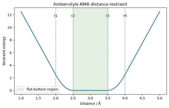
Note

In between r2 and r3, there is no force applied (though, here you’ll note for all restraints r2=r3, meaning the well is harmonic in all cases.)

With these boresch restraints generated, you are now ready to use them in your ABFE calculations!

Setting Up and Running Annihilation Simulations

For this activity, we will need two things to get started. The first is the equilibrated end-state files from the previous activity Equilibrating Endstates in ABFE Calculations (Tyk2); and the second is the Boresch restraint files generated in the activity Creating Boresch Restraints for ABFE Calculations (Tyk2). For your convenience, we have provided the necessary files below to get you started.

Attention

Update the download link to point to the finalized activity files once they are uploaded.

Choosing A Lambda Schedule

The first step in setting up an ABFE calculation is to define a lambda schedule. For the purposes of this activity we will use a simple linear lambda schedule with 11 windows.

Warning

A linear lambda schedule is usually not optimal for ABFE calculations, and ABFE calculations often need far more than 11 windows to converge. This activity is meant to demonstrate the basic steps of setting up and running an ABFE calculation, and is not intended to produce converged or realistic results.

The lambda schedule we will use is as follows:

Window  Lambda Value
---------------------
      0.0
      0.1
      0.2
      0.3
      0.4
      0.5
      0.6
      0.7
      0.8
      0.9
      1.0

Annihilation Simulation Setup

With a lambda schedule in place, we can now slowly annihilate the ligand from the equilibrated complex and binder end-states. Roughly, in both cases this involves starting from the end-state where \(\lambda = 0\) and gradually turning off the ligand’s interactions with its environment until it is fully decoupled at \(\lambda = 1\).

Annihilate (Binder)

&cntrl
imin = 1, 
maxcyc = 5000,
ncyc = 100, 
ntx = 1, 
ntmin = 2,
ntwe = 0, 
ntwr = 0, 
ntpr = 1000,
ntb = 1, 
ntp = 0,
cut = 10.0, 
ntr = 0,
ioutfm=1, 
ntxo=1,

ifsc            = 1
icfe            = 1

clambda         = REPLACE_WITH_LAMBDA
timask1         = ':1'
timask2         = ''
scmask1         = ':1'
scmask2         = ''
scalpha         = 0.5
scbeta          = 1.0

gti_cut         = 1
gti_output      = 1
gti_add_sc      = 25
gti_scale_beta  = 1
gti_cut_sc_on   = 8
gti_cut_sc_off  = 10
gti_lam_sch     = 1
gti_ele_sc      = 1
gti_vdw_sc      = 1
gti_cut_sc      = 2
gti_ele_exp     = 2
gti_vdw_exp     = 2
gti_syn_mass    = 0
gremd_acyc      = 1

gti_bat_sc      = -1
/

Annihilate (Complex)

&cntrl
imin = 1, 
maxcyc = 5000,
ncyc = 100, 
ntx = 1, 
ntmin = 2,
ntwe = 0,
ntwr = 0,
ntpr = 1000,
ntb = 1, 
ntp = 0,
cut = 10.0, 
ntr = 0,
ioutfm=1, 
ntxo=1,

ifsc            = 1
icfe            = 1

clambda         = REPLACE_WITH_LAMBDA
timask1         = ':1'
timask2         = ''
scmask1         = ':1'
scmask2         = ''
scalpha         = 0.5
scbeta          = 1.0

gti_cut         = 1
gti_output      = 1
gti_add_sc      = 25
gti_scale_beta  = 1
gti_cut_sc_on   = 8
gti_cut_sc_off  = 10
gti_lam_sch     = 1
gti_ele_sc      = 1
gti_vdw_sc      = 1
gti_cut_sc      = 2
gti_ele_exp     = 2
gti_vdw_exp     = 2
gti_syn_mass    = 0
gremd_acyc      = 1

gti_bat_sc      = -1
nmropt          = 1
/
&wt type = 'END', /
DISANG=rest.in
/

Above, we have included the mdin files used to annihilate the ligand in both the binder and the complex environments. Note. These mdin files contain a placeholder for the specific lambda value for each window. This is REPLACE_WITH_LAMBDA.

We will start by generating the lambda windows for both the binder and complex annihilation simulations. To do this, we will start with our simple lambda schedule defined above.

Start by creating a working_directory for these steps within the abfe_files directory. We will make separate directories for the binder and complex annihilation simulations within this folder.

mkdir working_dir
cd working_dir
mkdir binder complex

Next, we will use a bash for loop to generate the mdin files for each lambda window for both the binder and complex annihilation simulations.

# Binder Annhilation Windows
lambda_values=(0.0 0.1 0.2 0.3 0.4 0.5 0.6 0.7 0.8 0.9 1.0)
for i in ${!lambda_values[@]}
do
   lambda_value=${lambda_values[$i]}
   sed "s/REPLACE_WITH_LAMBDA/$lambda_value/g" ../binder_mdins/annhilate.mdin > binder/annihilate_lambda_${i}.mdin
done

# Complex Annhilation Windows
for i in ${!lambda_values[@]}
do
   lambda_value=${lambda_values[$i]}
   sed "s/REPLACE_WITH_LAMBDA/$lambda_value/g" ../complex_mdins/annhilate.mdin > complex/annihilate_lambda_${i}.mdin
done

Now, you should have 11 mdin files for both the binder and complex annihilation simulations, each corresponding to a different lambda window.

Now, we can proceed to run these lambda windows iteratively starting from the \(\lambda = 0\) window and moving to the next window using the output of the previous window as input.

We will start with the binder simulations. Here, we will use the equilibrated end-state files (provided with the activity files) as input for the first window (\(\lambda = 0\)), and then use the output of each window as input for the next window.

cd binder
# Run Lambda Windows Iteratively
for i in {0..10}
do
   if [ $i -eq 0 ]
   then
      # First window uses equilibrated end-state files
      pmemd.cuda -O -i annihilate_lambda_${i}.mdin -p  ../../topology/binder_ejm_31_hmr.parm7 -c ../../topology/binder_ejm_31_unrestrained.rst7 -o annihilate_binder_${i}.mdout -r annihilate_binder_${i}.rst7 -x annihilate_binder_${i}_traj.nc -ref ../../topology/binder_ejm_31_unrestrained.rst7
   else
      # Subsequent windows use output of previous window
      pmemd.cuda -O -i annihilate_lambda_${i}.mdin -p ../../topology/binder_ejm_31_hmr.parm7 -c annihilate_binder_$((i-1)).rst7 -o annihilate_binder_${i}.mdout -r annihilate_binder_${i}.rst7 -x annihilate_binder_${i}_traj.nc -ref annihilate_binder_$((i-1)).rst7
   fi
done

These commands will run the binder annilation simulations for each lambda window iteratively. These are minimizations, and thus are relatively quick to run.

For the complex simulations, we will follow the same procedure, except we also need to include the Boresch restraint rest.in file, as well as the lambda.sch file that defines how the restraints are scaled during the annihilation process.

This lambda.sch file controls how the Boresch restraints are scaled during the annihilation process to ensure that the ligand remains properly restrained as its interactions with the environment are turned off.

TypeRestBA, smooth_step2, symmetric, 1.0, 0.0

Warning

The lambda.sch file is essential for the proper scaling of Boresch restraints during the annihilation process. In the example TypeRestBA, smooth_step2, symmetric, 1.0, 0.0, the final two numbers indicate that the restraint is fully on at \(\lambda = 1.0\) and off at \(\lambda = 0.0\). If this file is not included, the restraints will be applied to the real state and then slowly turned off, which is exactly the opposite of what we want to achieve. This is a very common mistake when setting up ABFE calculations with Boresch restraints, and will lead to incorrect results.

Thus, we will copy these files into the complex working directory before running the simulations.

cd ../complex
cp ../../boresch_restraints/rest.in .
cp ../../boresch_restraints/lambda.sch .
# Run Lambda Windows Iteratively
for i in {0..10}
do
   if [ $i -eq 0 ]
   then
      # First window uses equilibrated end-state files
      pmemd.cuda -O -i annihilate_lambda_${i}.mdin -p ../../topology/target_ejm_31_hmr.parm7 -c ../../topology/complex_ejm_31_unrestrained.rst7 -o annihilate_complex_${i}_out.log -r annihilate_complex_${i}.rst7 -x annihilate_complex_${i}.nc -ref ../../topology/complex_ejm_31_unrestrained.rst7
   else
      # Subsequent windows use output of previous window
      pmemd.cuda -O -i annihilate_lambda_${i}.mdin -p ../../topology/target_ejm_31_hmr.parm7 -c annihilate_complex_$((i-1)).rst7 -o annihilate_complex_${i}.mdout -r annihilate_complex_${i}.rst7 -x annihilate_complex_${i}.nc -ref annihilate_complex_$((i-1)).rst7
   fi
done

These calculations will run relatively quickly, as they are minimizations. After this, we can move on to equilibrating the lambda windows.

Note

The mpirun commands below assume you are running on an interactive node or within an active batch allocation that provides access to 11 GPUs or GPU ranks.

Overview of the Outputs from An ABFE calculation

In the download or in your previous calculations, the production simulations were organized into two main phases: the binder phase and the complex phase.

Each phase consisted of multiple lambda windows, with each window having its own set of output files. For this activity, we will focus on analyzing the output log files (.mdout) generated during these calculations, as well as the replica exchange log files (remd_.log).

The mdout files contain detailed information about the energy components and other properties of the system at each step of the simulation. The remd log files provide information about the replica exchange attempts and outcomes, which can be useful for assessing the sampling efficiency across the lambda windows.

Specifically, the mdout files provide output that looks like this:

| TI region  1


NSTEP =   840250   TIME(PS) =    3361.000  TEMP(K) =   294.22  PRESS =     0.0
Etot   =    -33055.3946  EKtot   =      6151.6533  EPtot      =    -39207.0479
BOND   =         0.0000  ANGLE   =         0.0000  DIHED      =         3.6590
1-4 NB =        -0.0696  1-4 EEL =       -25.0360  VDWAALS    =      6648.6562
EELEC  =    -45834.2575  EHBOND  =         0.0000  RESTRAINT  =         0.0000
DV/DL  =        79.6779
TEMP0  =       298.0000  REPNUM  =              9  EXCHANGE#  =           8403
------------------------------------------------------------------------------

Softcore part of the system:      32 atoms,       TEMP(K)    =         269.57
SC_Etot=        41.8564  SC_EKtot=        22.7663  SC_EPtot   =        19.0901
SC_BOND=         6.4851  SC_ANGLE=        11.9679  SC_DIHED   =         6.5738
SC_14NB=         0.0000  SC_14EEL=         0.0000  SC_VDW     =        -5.9367
SC_EEL =         0.0000
SC_RES_DIST=     0.0000  SC_RES_ANG=       0.0000  SC_RES_TORS=         0.0000
SC_EEL_DER=      1.1039  SC_VDW_DER=     -15.3796  SC_DERIV   =       -14.2757
------------------------------------------------------------------------------


| TI region  2


NSTEP =   840250   TIME(PS) =    3361.000  TEMP(K) =   294.32  PRESS =     0.0
Etot   =    -33078.1609  EKtot   =      6128.8870  EPtot      =    -39207.0479
BOND   =         0.0000  ANGLE   =         0.0000  DIHED      =         3.6590
1-4 NB =        -0.0696  1-4 EEL =       -25.0360  VDWAALS    =      6648.6562
EELEC  =    -45834.2575  EHBOND  =         0.0000  RESTRAINT  =         0.0000
DV/DL  =        79.6779
TEMP0  =       298.0000  REPNUM  =              9  EXCHANGE#  =           8403
------------------------------------------------------------------------------

Note that this shows both the energy components, as well as the parts that come from the soft-core region of the system (i.e., the alchemically modified atoms).

Meanwhile, the remd log files provide output that looks like this:

# Replica Exchange log file
# numexchg is      12500
# REMD filenames:
#   remlog= remd_complex_ejm31.log
#   remtype= rem.type
# Rep#, Neibr#, Temp0, PotE(x_1), PotE(x_2), left_fe, right_fe, Success, Success rate (i,i+1)
...
# exchange     9032
   2    298.00 -39400.10 -39409.58 -Infinity     -1.79    T        0.87
   1    298.00 -39408.05 -39398.45      1.79    -10.40    T        0.35
   4    298.00 -39416.77 -39352.95     10.40    -22.46    F        0.06
   3    298.00 -39332.22 -39390.84     22.45    -33.45    F        0.01
   6    298.00 -39316.56 -39355.34     32.76    -36.65    F        0.00
   5    298.00 -39321.48 -39275.80     36.74    -34.91    F        0.00
   8    298.00 -39129.67 -39121.37     32.64    -25.37    F        0.00
   7    298.00 -39108.33 -39103.97     23.32    -13.02    F        0.00
  10    298.00 -39087.24 -39262.19     10.73     -3.20    F        0.07
   9    298.00 -39262.99 -39081.81      3.20     -0.44    F        0.74
  -1    298.00 -39197.79      0.00      0.03      0.00    F        0.00
# exchange     9033
  -1    298.00 -39438.52      0.00 -Infinity     -1.79    F        0.87
   3    298.00 -39467.30 -39324.55      1.79    -10.40    T        0.35
   2    298.00 -39314.20 -39456.10     10.40    -22.46    T        0.06
   5    298.00 -39259.84 -39308.14     22.45    -33.45    F        0.01
   4    298.00 -39282.02 -39223.52     32.76    -36.65    F        0.00
   7    298.00 -39248.23 -39241.31     36.74    -34.91    F        0.00
   6    298.00 -39220.57 -39210.90     32.64    -25.37    F        0.00
   9    298.00 -39378.26 -39145.48     23.32    -13.02    F        0.00
   8    298.00 -39137.02 -39358.97     10.73     -3.20    F        0.07
  11    298.00 -39218.70 -39185.63      3.20     -0.44    T        0.74
  10    298.00 -39185.17 -39218.08      0.03      0.00    T        0.00

Here, the final column is cumulative success rate for exchanges between adjacent replicas, which can be useful for assessing the efficiency of sampling across the lambda windows. Thus, the most important entry in this file is the final success rate for each pair of adjacent replicas.

Danger

It is important to ensure that the exchange success rates between adjacent replicas are reasonable (typically between 20-40%) to ensure adequate sampling across the lambda windows. If the success rates are too low, it may indicate that the lambda spacing is too large or that the system is not equilibrated properly.

To solve low success rates, there are a few strategies that can be employed:

Optimizing the existing lambda schedule to have smaller gaps between windows where success rates are low.
Increasing the simulation time for each window to allow for better equilibration and sampling.
Adding additional intermediate lambda windows to improve overlap between adjacent states. (Often, 24-48 windows are sufficient for ABFE calculations.)

Extracting Data using Amber2Dats

The first step in analyzing the ABFE calculations is to extract the relevant data from the simulation output files. For this, we will use the edgembar-amber2dats tool from the FE-Toolkit suite.

Hands-On Session 10: Perform AFE simulations for Absolute Binding, using free energy workflows

Learning objectives

Activities

Building Simulation Boxes for ABFE Calculations

Building the Ligand in the Aqueous Phase

Calculating the Number of Ions to Add

Building the Bound Protein-Ligand Complex

Optional: Applying Hydrogen Mass Reparationing (HMR)

Setting Up and Running End-State Equilibration

Equilibrating the Aqueous Endstates

Equilibrating the Complex Endstates

Determining Boresch Restraints

How to Determine Boresch Restraints

Setting Up and Running Annihilation Simulations

Choosing A Lambda Schedule

Annihilation Simulation Setup

Equilibrating the Lambda Windows

Binder Equilibration

Complex Equilibration

Running Production Simulations

Binder Production

Complex Production

Overview of the Outputs from An ABFE calculation

Extracting Data using Amber2Dats

Running Edgembar

Creating Free Energy HTML Reports

Understanding the Results