8. Hands-On Session 8: Analyze AFE simulation results using FE-ToolKit

Zeke Piskulich¹, Timothy Giese¹, and Darrin M. York¹

¹Laboratory for Biomolecular Simulation Research, Institute for Quantitative Biomedicine and Department of Chemistry and Chemical Biology, Rutgers University, Piscataway, NJ 08854, USA

8.1. Learning Objectives

Inspect the raw Amber alchemical simulation outputs (mdout, rem.log) that feed a binding free energy analysis.
Extract per-window energies into portable .dat files with edgembar-amber2dats.py, organized into the edge/env/stage/trial hierarchy.
Build edgembar inputs with DiscoverEdges and run BAR/MBAR analysis to produce portable HTML result files.

Interpret an Edgembar HTML edge report for a real Tyk2 ABFE calculation.
Diagnose simulation quality from the report’s error and warning metrics (equilibration, statistical inefficiency, phase-space overlap).
Compare BAR vs. TI estimates and inspect the convergence, dV/dL, and replica-exchange plots to judge whether a calculation is trustworthy.

Load edgembar results from a portable NetCDF file using the Edgembar Python API.
Extract BAR and TI free energies with their errors at the edge, stage, and trial levels.
Export replica-exchange statistics to build custom summaries in external programs.

Optimize lambda schedules for alchemical free energy calculations with fetkutils-tischedule.py.
Compare the three optimization criteria — phase-space overlap, acceptance ratio, and Kullback-Leibler divergence — to choose an appropriate method.
Evaluate an existing schedule with the --read flag and benchmark it against optimized schedules.
Interpret the schedule summary statistics and prediction/overlap plots to detect bottlenecks and judge schedule quality.

8.2. Activities

        flowchart LR

%% ===== extract simulation outputs to dats =====
A1["Amber AFE outputs<br/>mdouts<br/>rem.log<br/>rest.in"]
P1{{"<b>[§8.2.2.1]</b><br/>Extract per-lambda data<br/>edgembar-amber2dats.py"}}
O1["<b>[from §8.2.2.1]</b><br/>efep dat files<br/>edge/env/stage/trial dats"]
A1 --> P1
P1 --> O1

%% ===== build edge xml and run edgembar =====
P2{{"<b>[§8.2.2.2]</b><br/>Discover edges, write xml<br/>DiscoverEdges.py"}}
O2["<b>[from §8.2.2.2]</b><br/>Edge input<br/>edge_ejm31.xml"]
P3{{"<b>[§8.2.2.2]</b><br/>Run BAR/MBAR analysis<br/>edgembar_omp"}}
O3["<b>[from §8.2.2.2]</b><br/>Report script and data<br/>edge_ejm31.py<br/>edge_ejm31.html<br/>edge_ejm31.nc"]
O1 --> P2
P2 --> O2
O2 --> P3
P3 --> O3

classDef file fill:#fff7e6,stroke:#d98c00,stroke-width:1.5px,color:#111;
classDef program fill:#e8f1ff,stroke:#1f77b4,stroke-width:1.8px,color:#111;
classDef result fill:#eaf7ea,stroke:#2ca02c,stroke-width:1.5px,color:#111;
class A1 file;
class P1,P2,P3,P4,P5 program;
class O1,O2,O3,O4,O5 result;

In HandsOn9 and HandsOn10, you will learn how to run different variations of alchemical free energy simulations. In this HandsOn tutorial, you will learn how to analyze the results of these simulations using FE-Toolkit.

You will learn how to extract data from simulation output files, generate analysis reports for relative and absolute binding free energy calculations, and interpret the results.

For these calculations, you will use the following mamba environment. If you have previously used other amber modules in this session, you may need to run modules purge first to avoid conflicts with the FE-Toolkit environment.

module purge
unset PYTHONPATH
mamba activate ambertools

8.2.1. Accessing the Tutorial Files 

To get the tutorial data during the workshop, you can get a copy into your scratch with this command.

DataDir="/data/amber26/TutorialData/HandsOn8_FE_Toolkit"
TutorialDir="/scratch/$USER/TutorialData/HandsOn8_FE_Toolkit"
mkdir -p $TutorialDir
cp -r $DataDir/* $TutorialDir
cd $TutorialDir
cp -r input working_dir
cd working_dir

Danger

These files are nearly 50 gb. The limit of the DIPC home directory is 50 gb.

8.2.2. Getting Started with FE-Toolkit 

For this tutorial, we have provided the simulation output data from Absolute Binding Free Energy Calculations on Tyk2 for four ligands. In this tutorial, we will primarily use the files for the ligand ejm31; however, we have provided the other ligands as a reference (and as an opportunity for further practice).

To obtain the files, download this ABFE Simulation Output. This file is quite large - so it may take a few minutes to download.

Note

New users should review the FE-Toolkit quickstart.

Hint

The FE-Toolkit paper published by Giese and co-workers includes a significant Supporting Information that outlines much of what is included in this tutorial, as well as the underlying math driving these calculations. See the paper Giese et al.[1] for more information.

8.2.2.1. Simulation Outputs from Alchemical Free Energy Simulations with Amber 

The fundamental outputs from an Absolute Binding Free Energy (ABFE) calculation that we will be using are the following:

mdouts: These are Amber simulation output files that include energy information from each lambda window.
rem.log: These are Amber simulation output files that include information about replica exchange acceptances [2].
rest.in (ABFE Only): This file contains information about the Boresch restraints used in the Amber simulation.

Briefly - we will explore each of these files:

Amber AFE calculations write MDouts with entries that look something like this. They include information about the energies, the dV/dL value, which exchange you are on, as well as information about the soft-core potentials.

| TI region  1


NSTEP =   840250   TIME(PS) =    3361.000  TEMP(K) =   294.22  PRESS =     0.0
Etot   =    -33055.3946  EKtot   =      6151.6533  EPtot      =    -39207.0479
BOND   =         0.0000  ANGLE   =         0.0000  DIHED      =         3.6590
1-4 NB =        -0.0696  1-4 EEL =       -25.0360  VDWAALS    =      6648.6562
EELEC  =    -45834.2575  EHBOND  =         0.0000  RESTRAINT  =         0.0000
DV/DL  =        79.6779
TEMP0  =       298.0000  REPNUM  =              9  EXCHANGE#  =           8403
------------------------------------------------------------------------------

Softcore part of the system:      32 atoms,       TEMP(K)    =         269.57
SC_Etot=        41.8564  SC_EKtot=        22.7663  SC_EPtot   =        19.0901
SC_BOND=         6.4851  SC_ANGLE=        11.9679  SC_DIHED   =         6.5738
SC_14NB=         0.0000  SC_14EEL=         0.0000  SC_VDW     =        -5.9367
SC_EEL =         0.0000
SC_RES_DIST=     0.0000  SC_RES_ANG=       0.0000  SC_RES_TORS=         0.0000
SC_EEL_DER=      1.1039  SC_VDW_DER=     -15.3796  SC_DERIV   =       -14.2757
------------------------------------------------------------------------------


| TI region  2


NSTEP =   840250   TIME(PS) =    3361.000  TEMP(K) =   294.32  PRESS =     0.0
Etot   =    -33078.1609  EKtot   =      6128.8870  EPtot      =    -39207.0479
BOND   =         0.0000  ANGLE   =         0.0000  DIHED      =         3.6590
1-4 NB =        -0.0696  1-4 EEL =       -25.0360  VDWAALS    =      6648.6562
EELEC  =    -45834.2575  EHBOND  =         0.0000  RESTRAINT  =         0.0000
DV/DL  =        79.6779
TEMP0  =       298.0000  REPNUM  =              9  EXCHANGE#  =           8403
------------------------------------------------------------------------------

Amber also writes rem.log files which list the acceptances in exchanges between windows.

# Replica Exchange log file
# numexchg is      12500
# REMD filenames:
#   remlog= remd_complex_ejm31.log
#   remtype= rem.type
# Rep#, Neibr#, Temp0, PotE(x_1), PotE(x_2), left_fe, right_fe, Success, Success rate (i,i+1)
...
# exchange     9032
   2    298.00 -39400.10 -39409.58 -Infinity     -1.79    T        0.87
   1    298.00 -39408.05 -39398.45      1.79    -10.40    T        0.35
   4    298.00 -39416.77 -39352.95     10.40    -22.46    F        0.06
   3    298.00 -39332.22 -39390.84     22.45    -33.45    F        0.01
   6    298.00 -39316.56 -39355.34     32.76    -36.65    F        0.00
   5    298.00 -39321.48 -39275.80     36.74    -34.91    F        0.00
   8    298.00 -39129.67 -39121.37     32.64    -25.37    F        0.00
   7    298.00 -39108.33 -39103.97     23.32    -13.02    F        0.00
  10    298.00 -39087.24 -39262.19     10.73     -3.20    F        0.07
   9    298.00 -39262.99 -39081.81      3.20     -0.44    F        0.74
  -1    298.00 -39197.79      0.00      0.03      0.00    F        0.00
# exchange     9033
  -1    298.00 -39438.52      0.00 -Infinity     -1.79    F        0.87
   3    298.00 -39467.30 -39324.55      1.79    -10.40    T        0.35
   2    298.00 -39314.20 -39456.10     10.40    -22.46    T        0.06
   5    298.00 -39259.84 -39308.14     22.45    -33.45    F        0.01
   4    298.00 -39282.02 -39223.52     32.76    -36.65    F        0.00
   7    298.00 -39248.23 -39241.31     36.74    -34.91    F        0.00
   6    298.00 -39220.57 -39210.90     32.64    -25.37    F        0.00
   9    298.00 -39378.26 -39145.48     23.32    -13.02    F        0.00
   8    298.00 -39137.02 -39358.97     10.73     -3.20    F        0.07
  11    298.00 -39218.70 -39185.63      3.20     -0.44    T        0.74
  10    298.00 -39185.17 -39218.08      0.03      0.00    T        0.00

Lastly, in ABFE we use rest.in files to define Boresch restraints [3][4] (see the Boresch Restraint Tutorial) which hold the ligand in the protein while its interactions are decoupled from the rest of the system at \(\lambda=1\). These restraint files contain the 0-indexed atoms for a pairwise restraint, two angle restraints, and three dihedral restraints between the protein and the ligand.

&rst iat=1477,16,0
  r1=0.00000,r2=5.62704,r3=5.62704,r4=999.000,rk2=7.55, rk3=7.55/
&rst iat=1475,1477,16,0
  r1=0.00000,r2=72.87935,r3=72.87935,r4=180.000,rk2=49.42, rk3=49.42/
&rst iat=1477,16,11,0
  r1=0.00000,r2=101.39821,r3=101.39821,r4=180.000,rk2=58.05, rk3=58.05/
&rst iat=1479,1475,1477,16,0
  r1=-180.00000,r2=49.83917,r3=49.83917,r4=180.000,rk2=37.33, rk3=37.33/
&rst iat=1475,1477,16,11,0
  r1=-180.00000,r2=-74.38683,r3=-74.38683,r4=180.000,rk2=26.64, rk3=26.64/
&rst iat=1477,16,11,15,0
  r1=-180.00000,r2=31.60116,r3=31.60116,r4=180.000,rk2=26.79, rk3=26.79/

Note

Boresch restraints do work on the system during an ABFE calculation, and thus have to be included when analyzing them. These will be handled automatically by edgembar during this tutorial, but you can learn more on their impact on the free energy from (see the Boresch Contributions to the Free Energy Tutorial).

Take a look at the folders you downloaded above, and take a minute to look through these files. For each ligand, you have a rem.log file, many mdouts (1/\(\lambda\)-window), and one rest.in file. You would also normally have a trajectory output for at least the end-states; however, that is out of the scope for the present tutorial.

8.2.2.2. Generating Edgembar HTML Reports 

For this tutorial, you need to have edgembar installed. This can either be installed from source (https://gitlab.com/RutgersLBSR/fe-toolkit); however, there is also a Python distribution of edgembar (the component of FE-Toolkit we will be using) available on PyPI (pip install edgembar). More edgembar documentation is located here: https://rutgerslbsr.gitlab.io/fe-toolkit/edgembar/index.html

By default, the Edgembar program reads files that are program agnostic (dat files of the format column1: simulation time, column2: potential energy in kcal/mol). It generally expects these files to be split into the following substructure:

edge/
    env/
        stage/
            trial/

Note

edge: Represents the overall ABFE/RBFE calculation. The name comes from thinking of the calculation as an edge in an alchemical network.
env: This is the environment (e.g. aqueous, complex)
stage: This is what stage for that environment (for instance, if you have separate charge decoupling and vdw decoupling stages). With SmoothStep potentials [5], often there is just a single vdw stage.
trial: A subdirectory for each independent trial, usually named t1 t2 etc.

In a way, these are just labels. The important thing is that there is a single edge, two env values, and there can be arbitrarily many stage and trial values. Each of them represents a calculation, and a very raw sketch of their relationship would look like this:

\[\textbf{edge} = \sum_{\textbf{stages in target env}} \langle \textbf{trials in each stage} \rangle - \sum_{\textbf{stages in reference env}} \langle \textbf{trials in each stage} \rangle\]

In the case of using Amber as the simulation package, FE-Toolkit has built-in tools for generating this hierarchical structure, specifically edgembar-amber2dats.

For this - we will use a short bash script.

#!/bin/bash
#SBATCH --job-name=amber_gpu_run
#SBATCH --reservation=amber26
#SBATCH --nodes=1
#SBATCH --ntasks=1
#SBATCH --cpus-per-task=10
#SBATCH --mem=20000mb
#SBATCH --time=01:00:00
#SBATCH --qos=regular

source /scratch/amber26/software/miniforge3/etc/profile.d/conda.sh

edge=$1
mkdir -p dats

for env in {complex,binder};
do
    for stage in vdw;
    do
        for trial in {t1,t2};
        do
            echo "Extracting files for $edge/$env/$stage/$trial"
            mkdir -p dats/$edge/$env/$stage/$trial
            if [ "$env" == "complex" ];
            then
                edgembar-amber2dats.py -r $edge/$trial\_$env/remd_$edge.log --odir dats/$edge/$env/$stage/$trial/ --vba $edge/$trial\_$env/rest.in $(ls $edge/$trial\_$env/*mdout) &
            else
                edgembar-amber2dats.py -r $edge/$trial\_$env/remd_$edge.log --odir dats/$edge/$env/$stage/$trial/ $(ls $edge/$trial\_$env/*mdout) &
            fi
        done
    done
done

wait

Let’s explore the edgembar-amber2dats.py script quickly before running the script.

edgembar-amber2dats.py -h

There are a few important options that you should consider:

nan: What should MBAR do if an MBAR energy is ‘**’. The default is to revert to BAR analysis. Important for ABFE.
extra: Can add extra data to the edgembar output for decomposing DV/DL profiles. Its main use is plotting the contributions from electrostatics, 1-4 vdw interactions, etc.

For now, we will run without these.

Run the script for ejm31.

sbatch run_amber2dats.sh ejm31

Now - you’ll see lots of messages saying something along the lines of “Invalid energies within ejm31/t2_complex/complex_ejm31_1.00000.mdout; writing output for BAR. See the –nan option”. This is expected for ABFE, because for MBAR you evaluate the energy at every lambda point with respect to every other lambda point. For ABFE, this means that you often can be evaluating energies of clashes between the protein and the ligand (for instance, in a state where your ligand is fully decoupled.)

Now that these files are generated, take a moment to explore the dats folder. Note that it follows the rough scheme we described above of edge/env/stage/trial. Take a look at the files that you have there.

Now, we will use a small python script to create an xml for edgembar to work on.

#!/usr/bin/env python3
import edgembar
import os
from pathlib import Path

odir = Path("analysis")
s=r"dats/{edge}/{env}/{stage}/{trial}/efep_{traj}_{ene}.dat"

exclusions=None
# Load the dat files into an edges object
edges = edgembar.DiscoverEdges(s,
                                exclude_trials=exclusions,
                                target="complex",
                                reference="binder")

odir.mkdir(exist_ok=True)
for edge in edges:
    # Tell the edges about the shift from the boresch restraints.
    edge.SetVBAShift()
    # Reverse the order of lambdas (1->0) so that the sign is negative, which is what you would expect for an ABFE.
    for trial in edge.GetAllTrials():
        trial.reverse()


    fname = odir / (edge.name + ".xml")
    edge.WriteXml(fname)

A few things are happening in this file. The first is we are setting a template string to say how the dats folder is structured. Then we generate an edges object with DiscoverEdges. If you have outliers, you could potentially want to exclude those trials using the exclusions list (e.g. exclusions=[“t1”])

Now - run this script.

python DiscoverEdges.py

You’ll see a new analysis directory with xml files present for each of the transformations you ran amber2dats for previously (up to four!). These .xml files are the input to edgembar. Open one of them and you’ll see they have the same hierarchical structure of edges, environments, stages, and trials, along with the lambda values per trial (yes, you can use different schedules in every trial of every stage and environment), the path to the .dat files, and an optional constant shift in the free energy, if you used boresch restraints for that trial.

Next, run the actual BAR [6]/MBAR [7] calculation:

OMP_NUM_THREADS=8 edgembar_omp analysis/ejm31.xml --fwdrev --halves

Warning

edgembar and edgembar_omp are dependent on relative paths defined in the xml file. Thus, you must run it from outside of analysis.

The two options enable additional analysis for edgembar that we will discuss in a later part of this tutorial when we are looking at the HTML reports.

This script writes a Python script, which we can run as:

python analysis/ejm31.py
python analysis/ejm31.py --netcdf

Note that we are running it twice. If you only want the HTML report, the first command is enough; however, if you want a portable data file you can pass to other programs or parse yourself, the NetCDF option provides a self-contained file for you to do so.

Now you should see ejm31.html and ejm31.nc in your analysis directory!

8.2.3. FE-Toolkit HTML Reports 

The HTML report can be viewed here: Graph.html

8.2.3.1. Header 

Hint

** Troubleshooting Questions **

Do you have many errors and warnings?
Are you using a recent hash of edgembar?

The first thing you see in an HTML report is the header. It contains important information about the calculation, specifically which version of edgembar was used, what command called edgembar, and what errors and warnings were generated.

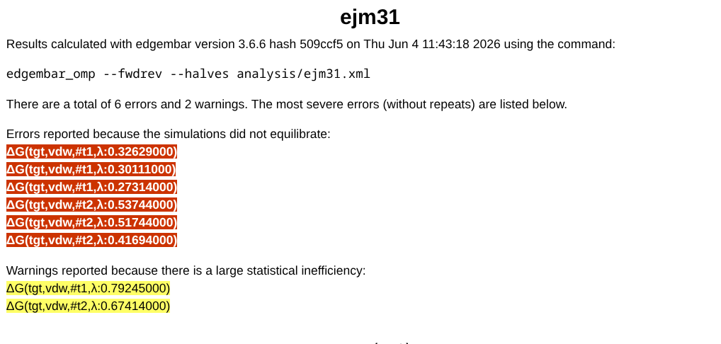
A few things are worth pointing out: every version of edgembar is given a unique hash (in the above image 3.6.6 H09ccf5), which can be useful for debugging.

Next, a summary of errors (shown in red) and warnings (shown in yellow) is included. Each entry is a hyperlink that jumps to the trial and lambda window where the issue was detected. These errors and warnings correspond to a few different aspects of a simulation’s quality. MOre details on the test that edgembar perfomrs to determine these errors and warings are availabe at FE-Toolkit edgembar guide: edgembar edge analysis.

Equilibration — whether too much of the simulation had to be discarded before reaching a stable production region. A simulation is flagged as unequilibrated if the discarded fraction exceeds --fmaxeq (default 0.5, i.e. 50%). In the report, this appears in the <f_eq> (fraction discarded) and N_eq (number of equilibration samples) columns of the per-trial data tables, and the convergence status is shown in the Conv? column.
Statistical inefficiency — how strongly correlated the samples in the production region are (larger is worse). A warning is raised if it exceeds 50; an error if it exceeds 100. In the report, this is the <g_prod> column (with g_ana for the analysis region and g for all data) of the per-trial data tables.
Number of independent samples — how many statistically independent samples remain in the production region (fewer is worse). This is computed as the number of samples divided by the statistical inefficiency. A warning is raised if there are fewer than 100; an error if there are fewer than 50. In the report, this is the N_ana column (with N for all data) of the per-trial data tables.
Phase-space overlap — how well a lambda window overlaps with its next neighbor (lower is worse). A warning is raised if the overlap is less than 0.25; an error if it is less than 0.15. In the report, this is the S column of the per-trial data tables.
Reweighting entropy — the effective sampling overlap with the next neighboring window (lower is worse). A warning is raised if it is less than 0.6; an error if it is less than 0.4. In the report, this is the RE column of the per-trial data tables.

How the production region is identified — and therefore which simulations get flagged as unequilibrated — can be tuned with the following analysis options to edgembar:

--ptol — the significance level (p-value) for the test that detects the production region. Larger values discard more data as equilibration.
--dtol — if the first-half and last-half means are within this tolerance (default: 0.1 kcal/mol), the window is treated as equilibrated.
--fmaxeq — the maximum fraction of a simulation that may be discarded as equilibration (default: 0.5).
--ferreq — flag a simulation as an error if more than this fraction would be discarded (default: equal to --fmaxeq).
--no-auto — disable automatic equilibration detection entirely and analyze all samples from --fstart to --fstop.

8.2.3.2. Objective Function 

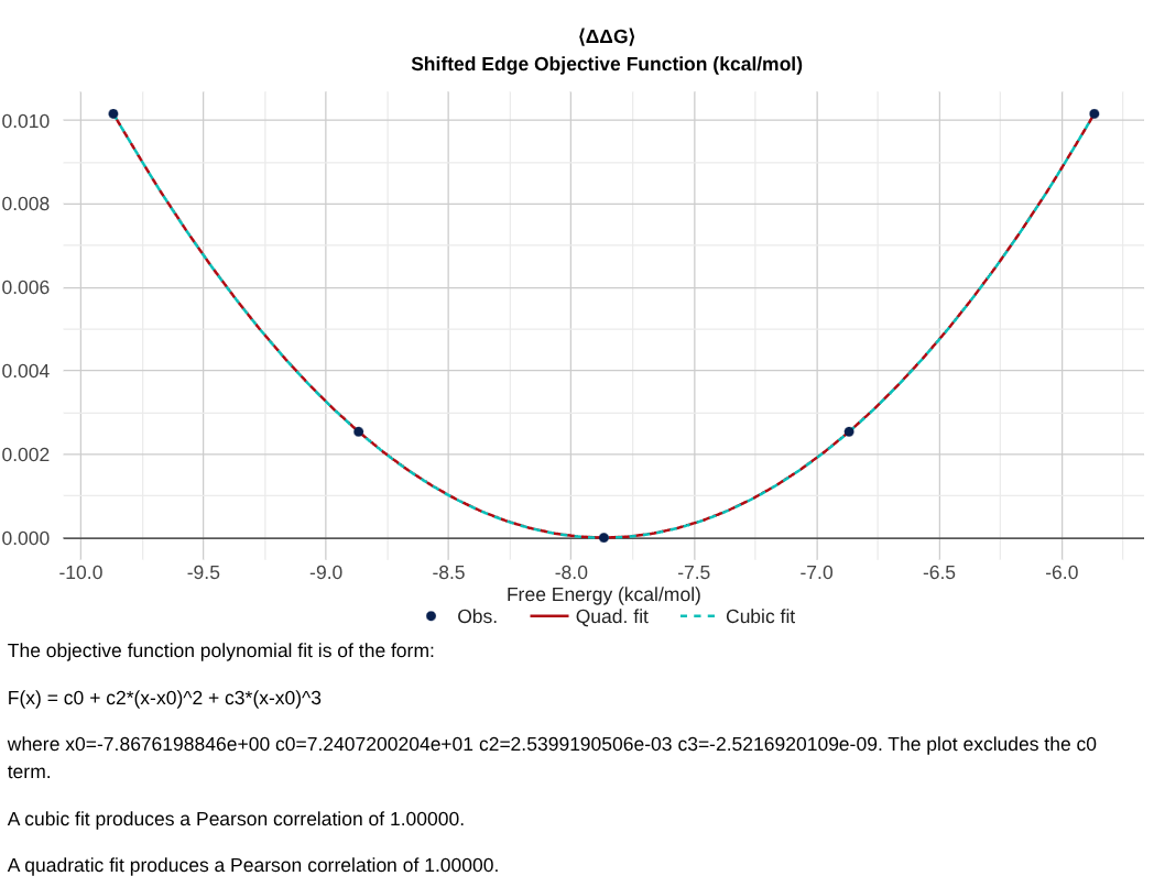
The next plot you see in the edge report is the “Shifted Edge Objective Function”, which shows the objective function that was minimized across all samples of an edge to obtain a specific final value shown on the x-axis. The minimum value corresponds to an unconstrained variational solution of the MBAR or BAR equations. Other values correspond to constrained variational solutions (where the constraint is for the x-axis value).

Unless there are problems with the simulation data, this plot should be a quadratic function that can be pre-computed for each edge and used to efficiently solve the network-wide set of equations. The curve is fit to a quadratic and cubic function using the 5 points indicated. These fits should produce Pearson correlations greater than 0.99, and the cubic terms should be less than \(10^{-5}\).

Note

The edge objective function is only relevant for network-wide analysis; it does not affect any aspect of the edge report. The edgembar-WriteGraphHtml.py script performs network-wide analysis, and by default solves for the node free energies using a quadratic approximation for the edge objective functions. This is often sufficient. One can use --solver=nonlinear or --solver=mixed to solve with the cubic fits. The mixed version solves with the cubic fits but then does bootstrap error calculations using the quadratic fits. This --solver=nonlinear or --solver=mixed is not recommended because it is very slow and not necessarily more accurate unless there were severe discrepancies in the objective function fits shown in the edge report.

8.2.3.3. Overall results 

Hint

** Troubleshooting Questions **

Do your BAR and TI results in the table agree?
How far does your fwdrev analysis deviate from production?
Is there a significant trend in your first and last half analysis?

The next set of data you’ll see is a summary table of the free energy values, and-if you ran edgembar with - -fwdrev and - -halves -a pair of timeseries figures above it. The “Fwd & Rev Analysis” figure shown on the left compares the free energies calculated from the first X% of the data to those calculated from the last X% of the data. The “First- & Last-Half Analysis” figure shown on the right which excludes X% of the simulation from start as equilibration, and splits the remaining 100-X% of data into two halves and compares the free energy from each half.

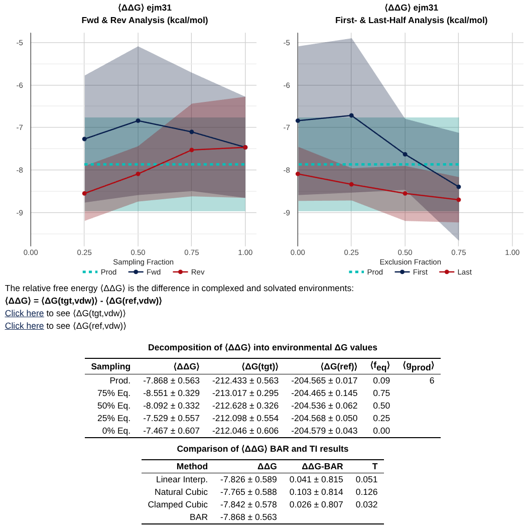
Fwd & Rev and First- & Last-Half analysis

Most important is the table at the bottom, which gives you a summary of the values from analysis with Bennett’s Acceptance Ratio (BAR) [6], and Thermodynamic Integration (TI) [8].

Note

A key debugging tool is to check agreement between BAR and TI. If these values do not agree - it suggests a problem with either equilibration, replica exchange acceptances, or alchemical pathway.

The shaded bands around the lines are 95% confidence intervals, obtained by scaling the standard error of the mean by 1.96 - a factor that tends to underestimate the true confidence interval. When the fwdrev or halves lines separate from each other by more than these bands, it usually points to a problem with the simulation or its equilibration. In that situation, it helps to inspect the trajectory directly: the plots alone may not reveal whether the start of the simulation was insufficiently equilibrated or if something catastrophic happened in the middle to simulate it incorrectly near the end.

8.2.3.4. DV/DL Profiles and Replica Exchanges 

Hint

** Troubleshooting Questions **

Is your DV/DL profile smooth? Does it have weird discontinuities?
Are there big differences in your DV/DL profiles between trials?
Does your replica exchange acceptance ratio ever approach a low number (< 0.2?)

The next key set of plots that are found are the DV/DL profile, and the Replica Exchange Acceptance Ratios.

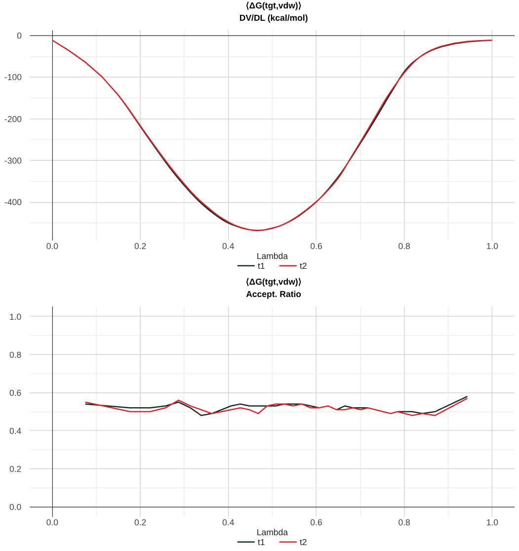
In the above image, you can see a well-converged DV/DL profile. Note that the trials track pretty well along each other.

Recall that the dV/dL profile is intrinsically linked to the free energy by the equation:

\[\Delta G = \int_0^1 \left\langle \frac{\partial V(\mathbf{x}; \lambda)}{\partial \lambda} \right\rangle_{\lambda} d\lambda\]

Note

For ABFE calculations, the dV/dL profile is shifted by a constant number. This number originates from the correction to the free energy that comes from Boresch Restraints. Determining the Boresch Restraint Contribution to the Free Energy.

Now, the replica exchange acceptance ratio is included in the second plot, and it gives you information for each pair of lambda windows what percentage of exchanges were accepted. Here, the value of 0.5 suggests that there were sufficient exchanges.

8.2.3.5. Data Tables 

Hint

** Troubleshooting Questions **

Did a lot of simulation data get thrown out when selecting production regions?
Did this trial have many (or most) of the warnings?
Do you have single passes and round trips in your calculation?

The next major section of the file is a set of tables (per environment and per trial) that give summary information about the free energy calculation as a function of lambda.

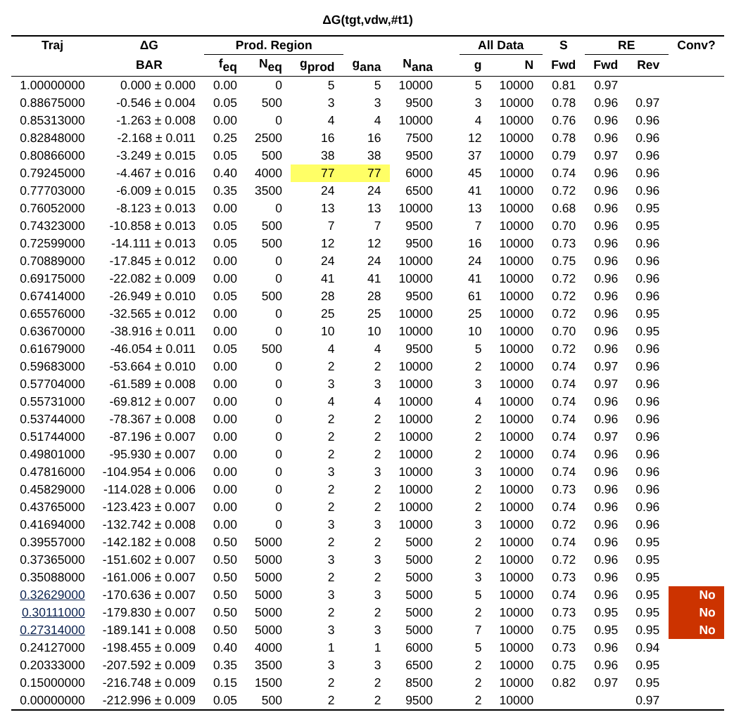
The columns of this trial data table are separated into three sections that report the same statistics computed over different subsets of the data. One section reports the statistics computed using only the “production region” (columns ending in _prod, such as <g_prod>). Another section reports the statistics computed when “all data” is considered (columns such as g). The “ana” section (columns ending in _ana, such as g_ana) reports the statistics for the data that are actually being analyzed, which could be either the “all data” or the “production region” depending on the analysis options used.

There is also a replica exchange data table that provides the data included in the acceptance ratio plot.

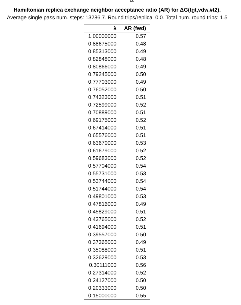
The header of this table includes a few additional useful pieces of information:

Average single pass num. steps: The amount of time it takes for a replica to exchange all the way \(0 \rightarrow 1\) or \(1 \rightarrow 0\)
Round trips/replica: Total number of round trips divided by the number of replicas.
Total num. round trips: The number of times a replica traverses \(0 \rightarrow 1 \rightarrow 0\) or \(1 \rightarrow 0 \rightarrow 1\)

8.2.3.6. Troubleshooting 

Hint

** Troubleshooting Questions **

Does the window look converged?
What is the scale of the dependence on the y-axis of the block average

Each lambda window that has a warning also gets a special section which includes information about the convergence of that window.

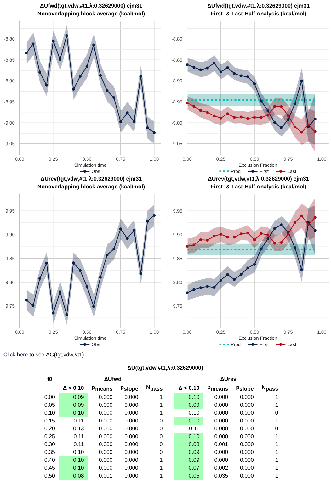
This shows plots of block averages over time, data tables, etc that can be used for additional debugging.

8.2.3.7. Wrapping Up 

In this activity, you walked through the pieces of an HTML report. Go through the troubleshooting questions at the top of each relevant section with that report. Does this pass as an okay simulation?

For the next tutorial, change directories into the API subdirectory.

cd ../API

8.2.4. Introduction to the Edgembar Python API 

Data generated from the edgembar package in FE-Toolkit Giese et al.[1] is typically stored in one of three sources. The first is an edge Python file (e.g. edge_ejm31.py), the second is a NetCDF file (e.g. edge_ejm31.nc), and the third is an HTML report (e.g. edge_ejm31.html). Each serves a particular purpose; however, when developing outside analysis tools that interact with them, the choice can make a significant impact. For instance, the .py file is dependent on relative paths, so if you move it to a different directory, then it will no longer be able to generate an HTML report. The HTML report includes a significant amount of information and is portable; however, it’s challenging to parse in Python. Therefore, the NC file exists as a portable (and parseable) solution.

To start, download the NetCDF file for an ABFE run on ejm31: This file

from __future__ import annotations

import argparse
from pathlib import Path

from edgembar.HtmlUtils import GetReplExchData
from edgembar.NcIO import LoadEdgeNc


def format_energy(value: float, error: float) -> str:
    return f"{value:8.3f} +- {error:6.3f} kcal/mol"


def print_bar_summary(label: str, obj, prod_data) -> None:
    value, error = obj.GetValueAndError(prod_data)
    print(f"{label:<28} {format_energy(value, error)}")


def print_ti_summary(edge) -> None:
    ti_data = edge.GetTIValuesAndErrors()
    if ti_data is None:
        print("TI estimates: unavailable")
        return

    print("TI estimates:")
    for method in ("Linear", "Natural", "Clamped"):
        if method in ti_data:
            value, error = ti_data[method]
            print(f"  {method:<8} {format_energy(value, error)}")


def print_message_summary(edge) -> None:
    messages = edge.GetErrorMsgs()
    errors = [msg for msg in messages if msg.iserr]
    warnings = [msg for msg in messages if not msg.iserr and msg.kind != "outlier"]

    print(f"Errors:   {len(errors)}")
    print(f"Warnings: {len(warnings)}")


def print_trial_summary(trial, prod_data) -> None:
    print_bar_summary(f"      trial {trial.name}", trial, prod_data)

    rem_data = GetReplExchData(trial)
    if rem_data is None:
        return

    single_pass = rem_data["Average single pass steps:"]
    trips_per_replica = rem_data["Round trips per replica:"]
    total_round_trips = rem_data["Total round trips:"]
    print(
        " " * 8
        + "RE summary: "
        + f"single-pass={single_pass:.1f}, "
        + f"round-trips/replica={trips_per_replica:.2f}, "
        + f"total-round-trips={total_round_trips:.1f}"
    )


def build_parser() -> argparse.ArgumentParser:
    parser = argparse.ArgumentParser(
        description="Read an EdgeMBAR .nc file and print a simple energy summary."
    )
    parser.add_argument("edge_nc", type=Path, help="Path to an EdgeMBAR NetCDF file")
    return parser


def main() -> None:
    args = build_parser().parse_args()

    if args.edge_nc.suffix != ".nc":
        raise SystemExit("Expected a NetCDF edge file ending in .nc")
    if not args.edge_nc.exists():
        raise SystemExit(f"File not found: {args.edge_nc}")

    edge = LoadEdgeNc(str(args.edge_nc))
    prod_data = edge.results.prod

    print(f"Edge: {edge.name}")
    print_bar_summary("edge", edge, prod_data)
    print_ti_summary(edge)
    print_message_summary(edge)
    print()

    for env in edge.GetEnvs():
        print_bar_summary(f"  env {env.name}", env, prod_data)
        for stage in env.stages:
            print_bar_summary(f"    stage {stage.name}", stage, prod_data)
            for trial in stage.trials:
                print_trial_summary(trial, prod_data)
        print()


if __name__ == "__main__":
    main()

Above is a Python script that you can use to access the data that you were looking at in the HTML report from the NetCDF file.

The key steps are:

Load an edge with LoadEdgeNc
The free energy is obtained by running edge.GetValueAndError(edge.results.prod) (or stage, or env, or trial)
The replica exchange information is provided by GetReplExchData(trial)

For the next tutorial, change directories into the LambdaSchedules subdirectory.

cd ../LambdaSchedules

mamba deactivate
module load Amber/25.0-foss-2022a-AmberTools-25-CUDA-12.1.1-DeePMD

8.2.5. Introduction to Optimizing Lambda Schedules 

8.2.5.1. Why the Lambda Schedule Matters 

In alchemical free energy simulations, the coupling parameter \(\lambda\) defines an artificial pathway between two thermodynamic states, such as ligand A \(\rightarrow\) ligand B in an RBFE calculation, or an interacting ligand \(\rightarrow\) noninteracting dummy state in an ABFE calculation. Although the free energy is a state function, the reliability of alchemical free energy simulations depends on the ability to robustly sample phase space along an artificial coordinate \(\lambda\). In methods like Alchemical Enhanced Sampling (ACES), efficiency is driven by Hamiltonian replica exchange, whose success is highly correlated with the degree of phase space overlap between adjacent \(\lambda\)-windows. Traditional \(\lambda\)-spacing schedules often create bottlenecks-intervals with very low exchange probabilities-that stall sampling and prevent the necessary traversal of conformational states. Optimizing the \(\lambda\)-schedule is necessary to equalize these overlaps, ensuring a high throughput of end-to-end “single passes” and “round trips” across the alchemical path. By tailoring the schedule to the specific phase space of a system, optimization eliminates these bottlenecks, leading to significantly more precise and robust free energy estimates.

8.2.5.2. Optimization Methods: PSO, AR, KL 

Optimized lambda scheduling uses short preliminary, or “burn-in,” simulations to estimate how well different lambda states overlap. These data are used to build a two-dimensional map, \(O(\lambda,\lambda')\), that predicts the overlap or exchange behavior between any pair of lambda values. For a fixed number of lambda windows, the optimized schedule is chosen (with the endpoints fixed at \(\lambda=0\) and \(\lambda=1\)) so that the variance of the overlap index across adjacent intervals is minimized, making the overlap between neighboring windows as uniform as possible.

Opt-PSO: Optimized Phase-Space Overlap. Opt-PSO directly optimizes the phase-space overlap between neighboring lambda windows. For each lambda state, short simulations generate samples from that state. Energy differences between pairs of lambda states are computed and approximated as distributions. The overlap between these distributions gives an overlap index \(O_{ij}\), where larger values indicate better similarity between ensembles.

The discrete overlap values from burn-in simulations are interpolated into a continuous function \(O(\lambda,\lambda')\). The first and last windows are fixed at \(\lambda=0\) and \(\lambda=1\), while the internal lambda values are adjusted to minimize the variance in nearest-neighbor overlaps. In simple terms, Opt-PSO tries to make every adjacent lambda pair share comparable statistical overlap; since PSO and the H-REMD acceptance ratio are strongly correlated, this also tends to produce comparably efficient replica exchange between every pair of neighboring windows.

Opt-KL: Optimized Kullback-Leibler Divergence. Opt-KL uses the Kullback-Leibler divergence as the measure of dissimilarity between neighboring lambda ensembles. KL divergence measures how different one probability distribution is from another. A symmetric KL divergence can be used so that the difference between state \(i\) and state \(j\) is treated consistently in both directions. When two distributions are very similar, the KL divergence is small; when they differ strongly, the KL divergence becomes large.

To use KL divergence in a scheduling procedure similar to Opt-PSO, the divergence is converted into a KL-based overlap index that decreases as the divergence grows. The resulting continuous map is optimized in the same general way: choose lambda values that make the neighboring intervals more uniform. In practice, the KL method is no better than PSO.

Opt-AR: Optimized Acceptance Ratio. Opt-AR optimizes the lambda schedule using the replica-exchange acceptance ratio directly. Instead of estimating overlap through distribution similarity, it estimates the probability that replicas at two lambda states would exchange according to the Metropolis criterion. The average exchange probability becomes the optimization index.

Because exchange acceptance is the practical quantity that controls how efficiently walkers move through lambda space, Opt-AR is especially intuitive for HREMD-based workflows, and its underlying acceptance-ratio map tends to decay monotonically away from the diagonal, which can make it the most predictable choice when a schedule needs to be selected automatically. The final optimization is analogous to Opt-PSO: construct a continuous acceptance-ratio map and adjust the internal lambda points so that neighboring exchange probabilities are more balanced across the full lambda path.

8.2.5.3. Running fetkutils-tischedule.py 

8.2.5.3.1. Input Files 

The lambda schedule optimization tool reads the efep_*_*.dat files produced from your burn-in simulation by edgembar-amber2dats.py (see Analyzing Free Energy Calculations with FE-Toolkit). These files must follow a specific naming convention and format:

File naming:

dvdl_<lambda>.dat: the \(\partial V/\partial\lambda\) time series produced at lambda. fetkutils-tischedule.py uses the presence of these files to automatically detect which lambda values were sampled during the burn-in.
efep_<lambda1>_<lambda2>.dat: potential energies evaluated at lambda2, using configurations sampled from the trajectory run at lambda1.

File format (efep_*_*.dat): Two-column, whitespace-separated values

Column 1: Simulation time (in step numbers)
Column 2: Potential energy (kcal/mol)

Example file structure:

To obtain the most reliable schedule, you want a complete matrix of energy evaluation files. This means:

For every trajectory generated at lambda value \(\lambda_i\)
You have energy evaluations at all lambda values \(\lambda_j\) (where \(j\) ranges from 0 to \(N_{windows}\))

For example, if you have 16 initial lambda windows (0 to 15), you would ideally have 16 × 16 = 256 total efep_*_*.dat files.

Note

The diagonal files (efep_i_i.dat) represent energies evaluated at the same lambda as the simulation, and are required to compute the PSO/AR/KL indices for that window. Off-diagonal files are the cross-evaluations needed for the two-dimensional overlap map, as well as for MBAR analysis.

8.2.5.3.2. Optimizing a Schedule 

For this activity, we provide a set of burn-in energy files (the efep_*_*.dat files for ligand ejm_31 bound to Tyk2), already generated with edgembar-amber2dats.py (see Analyzing Free Energy Calculations with FE-Toolkit).

Inside, you will find the dats/ejm_31/complex/vdw/t1/ directory, organized following the same edge/environment/stage/trial layout that edgembar-amber2dats.py produces from your Amber AFE outputs (mdouts and rem.log). This directory contains the burn-in energy files that fetkutils-tischedule.py reads.

The FE-ToolKit fetkutils-tischedule.py utility implements the three optimization criteria described above (Opt-PSO, Opt-AR, and Opt-KL), each estimated from a short burn-in simulation. Choose one of the three:

Acceptance Ratio (AR)

fetkutils-tischedule.py --opt 32 --ar \
    --plot opt_ar_32.png -o opt_ar_32.txt \
    dats/ejm_31/complex/vdw/t1/

Phase Space Overlap (PSO)

fetkutils-tischedule.py --opt 32 --pso \
    --plot opt_pso_32.png -o opt_pso_32.txt \
    dats/ejm_31/complex/vdw/t1/

Kullback-Leibler (KL)

fetkutils-tischedule.py --opt 32 --kl \
    --plot opt_kl_32.png -o opt_kl_32.txt \
    dats/ejm_31/complex/vdw/t1/

--pso: Optimize based on the phase space overlap index
--ar: Optimize based on the predicted replica exchange acceptance ratio (recommended)
--kl: Optimize based on the symmetrized Kullback-Leibler divergence
--opt N: Optimize to N lambda windows (commonly 8-24; more windows improve exchange statistics and free energy precision at increased computational cost)
--sym: Force the schedule to be symmetric about \(\lambda=0.5\), halving the number of free parameters
--ssc: (optional) Restrict the schedule to the analytic SSC(\(\alpha\)) smoothstep family instead of optimizing each lambda value independently; 1 parameter with --sym, otherwise 2 (--alpha0/--alpha1)
--maxgap VALUE: Maximum allowed spacing between adjacent lambda values (default 1.0)
--plot FILE: Write a two-panel figure: the predicted index vs. lambda, and the full 2D overlap map with the schedule overlaid
-o FILE or --out FILE: Write the optimized lambda schedule to file

8.2.5.3.3. Evaluating an Existing Schedule 

To predict the PSO/AR/KL profile of a schedule you already have, without optimizing, pass the schedule file to --read. The file should contain one lambda value per line:

This is useful whenever you already have a schedule and want to see how it performs. For example, if you have a custom schedule from some other method — you can predict its AR/PSO/KL statistics with the same --read command and compare them directly against the optimized schedules produced with --opt.

To try this, save the schedule you want to evaluate as a text file with one lambda value per line. For example below is a 24-window evenly spaced (linear) schedule. Copy it into a file named production_schedule.txt in your working directory. Then run with fetkutils-tischedule.py --read flag above to predict this linear schedule’s statistics.

fetkutils-tischedule.py --read production_schedule.txt --pso \
    --plot production_schedule_pso.png \
    dats/ejm_31/complex/vdw/t1/

--read FILE: Evaluate an existing schedule without optimizing. FILE should contain one column; the rows are the lambda values.
--pso, --ar, or --kl: Choose the metric to evaluate
--plot FILE: Generate the two-panel plot of the metric profile

8.2.5.4. Interpreting the Results 

8.2.5.4.1. The Schedule File and Summary 

The output file (e.g., opt_ar_32.txt) contains the optimized lambda schedule, one value per line formatted to 8 decimal places. For example, the 32-window AR-optimized schedule for the ejm31 complex looks like:

These values represent the lambda schedule to use in your production simulations. Note:

First value is always 0.0
Last value is always 1.0

Every run of fetkutils-tischedule.py also prints a summary of the schedule to the terminal, including the maximum gap between windows and the mean, standard deviation, maximum, and minimum of the chosen index across all intervals:

Max Gap:    0.1636
Mean Value: 0.4813
Std Value:  0.0001
Max Value:  0.4815
Min Value:  0.4812

Read this summary as follows:

Std Value is the key indicator of schedule quality. Here it is 0.0001, meaning the predicted acceptance ratio is essentially identical across all 31 intervals-the schedule is very well optimized, with no bottlenecks.
Mean Value (0.4813) is the average predicted index across the intervals; every adjacent pair of windows is predicted to exchange with roughly 48% probability.
Min Value (0.4812) is the weakest interval in the schedule. Here it is essentially equal to the mean, so no interval is a bottleneck. A Min Value that dropped toward zero would flag an interval where the windows are spaced too far apart and should be subdivided by increasing --opt.
Max Gap (0.1636) is the largest spacing between adjacent lambda values-here the first interval, from \(\lambda=0\) to \(\lambda=0.16355\), where the phase space changes slowly enough that a wide step still maintains high overlap.

8.2.5.4.2. The Prediction Plot 

The --plot option writes a two-panel figure that summarizes the same information visually. The figure below is the plot for the 32-window AR-optimized schedule above (opt_ar_32.png):

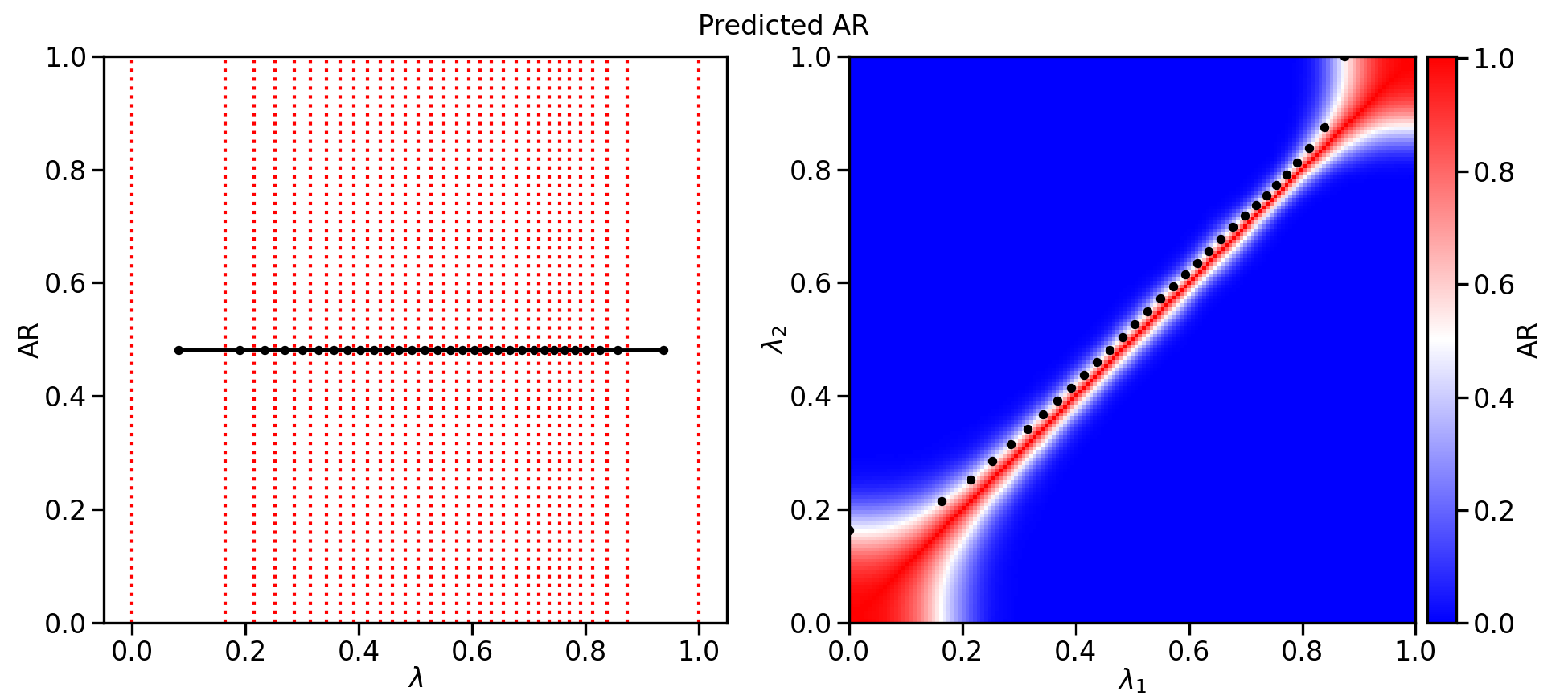
Predicted acceptance ratio for the optimized 32-window schedule

Left panel — predicted index vs. lambda. Each black point is the predicted index (here the acceptance ratio, AR) at the midpoint of an interval, and the red dotted vertical lines mark the 32 optimized lambda windows. The black profile is essentially flat which shows every adjacent pair of windows has the same predicted acceptance ratio, so there is no bottleneck. A poor schedule would instead show dips in this profile, marking intervals where exchange stalls.

Right panel — the two-dimensional overlap map. This is the interpolated map \(O(\lambda_1,\lambda_2)\): red indicates high acceptance/overlap (near the diagonal, where two states are similar) and blue indicates low acceptance/overlap (states too far apart to exchange). The black dots are the adjacent-window pairs \((\lambda_i,\lambda_{i+1})\) of the optimized schedule. Because the optimization equalizes the index, the dots all lie along the same narrow red band just off the diagonal — every neighboring pair sits at the same, high acceptance. If a schedule were poorly spaced, some black dots would stray outward into the pale or blue region, revealing a bottleneck interval.

8.3. Alternative Methods

pymbar - a python package for MBAR analysis. See the pymbar documentation for more information: https://pymbar.readthedocs.io/en/latest/

8. Hands-On Session 8: Analyze AFE simulation results using FE-ToolKit

8.1. Learning Objectives

8.2. Activities

8.3. Alternative Methods

8.4. References