13. Hands-On Session 13: Using AmberStudio to Perform Alchemical Free Energy Simulations
13.1. Learning Objectives
Learn about the basic components of AmberStudio.
Learn about the differences between Artifacts, WorkNodes, Flows, and Pipelines.
Learn what files are required for an AmberStudio ABFE calculation.
Set up and prepare files for ABFE on Tyk2 inhibitors.
Learn how to set up a free MD calculation with AmberStudio.
Learn how to run an equilibration with AmberStudio.
Learn how to connect multiple flows together with AmberStudio.
Learn what files are required for an AmberStudio ABFE calculation.
Set up and prepare files for ABFE on Tyk2 inhibitors.
Learn what files are required for an AmberStudio ABFE calculations
Set-up and prepare files for ABFE on Tyk2 inhibitors
13.2. Activities
        flowchart LR

%% ===== inputs =====
A1["Input structures<br/>binder_ejm31.pdb<br/>target_ejm31.pdb"]

%% ===== concepts =====
C1{{"<b>[§13.2.1]</b><br/>Concepts: Artifacts<br/>WorkNodes, Flows, Pipelines"}}

%% ===== ligand parameters =====
P2{{"<b>[§13.2.2]</b><br/>Generate ligand parameters<br/>ParametrizeBinderBCC"}}
O2["<b>[from §13.2.2]</b><br/>Ligand parameters<br/>binder.mol2 / .lib / .frcmod"]

%% ===== build systems =====
P3{{"<b>[§13.2.3]</b><br/>Build solvated systems<br/>FlowBuild"}}
O3["<b>[from §13.2.3]</b><br/>Built systems<br/>complex/binder .parm7 / .rst7"]

%% ===== free-MD =====
P4a{{"<b>[§13.2.4.1]</b><br/>Equilibrate system<br/>FlowRoeRelax"}}
P4b{{"<b>[§13.2.4.2]</b><br/>Append free MD<br/>MDRun"}}
O4["<b>[from §13.2.4]</b><br/>Equilibrated system<br/>MD trajectory .nc"]

%% ===== ABFE =====
P5{{"<b>[§13.2.5]</b><br/>Absolute binding free energy<br/>FlowABFEProduction"}}
O5["<b>[from §13.2.5]</b><br/>Binding free energy<br/>delta-G report"]

%% ===== RBFE =====
P6a{{"<b>[§13.2.6.1]</b><br/>Build RBFE edges<br/>AmberStudio"}}
P6b{{"<b>[§13.2.6.2]</b><br/>Run RBFE edges<br/>AmberStudio"}}
O6["<b>[from §13.2.6]</b><br/>Relative binding free energy<br/>delta-delta-G"]

C1 --> A1
A1 --> P2
P2 --> O2
O2 --> P3
P3 --> O3
O3 --> P4a
P4a --> P4b
P4b --> O4
O4 --> P5
P5 --> O5
O4 --> P6a
P6a --> P6b
P6b --> O6

classDef file fill:#fff7e6,stroke:#d98c00,stroke-width:1.5px,color:#111;
classDef program fill:#e8f1ff,stroke:#1f77b4,stroke-width:1.8px,color:#111;
classDef result fill:#eaf7ea,stroke:#2ca02c,stroke-width:1.5px,color:#111;
class A1 file;
class C1,P2,P3,P4a,P4b,P5,P6a,P6b program;
class O2,O3,O4,O5,O6 result;
13.2.1. Introduction to AmberStudio
AmberStudio is a platform for running Molecular Dynamics simulations with Amber. One of the challenges with running complex calculations with Amber is the need to run calculations in many stages (e.g. minimization, density equilibration, heating, equilibration, production) often resulting in more than ten MD input files for a single calculation. AmberStudio allows you to generate custom workflows that automate a significant portion of this process.
We will briefly outline the basic components of AmberStudio.
13.2.1.1. Artifacts
Artifacts are the basic file units passed between WorkNodes. These are usually file-type objects (e.g. ligand topologies, PDB files, NC trajectory files, analysis HTML files).
Below you can see an example of a BinderLigandPDB artifact (which is a PDB of a ligand that binds to a protein).
from amberstudio.artifacts import BinderLigandPDB

artifact = BinderLigandPDB("binder_ejm31.pdb")
print(artifact.filepath)
13.2.1.2. WorkNodes
WorkNodes are the basic unit of work within AmberStudio. Generally, each WorkNode performs one task, transforming its input Artifact objects into output Artifact objects.
In the example below, you can see a WorkNode that applies PDB4Amber to a protein PDB.
This WorkNode takes an input PDB file, applies PDB4Amber to it, and then produces a cleaned PDB as an output Artifact.
from amberstudio.worknodes import PDB4Amber

worknode = PDB4Amber(
    wnid="clean_target",
    nohyd=True,
    skippable=True,
)
print(worknode.id)
WorkNodes specify which types of input artifacts they expect and which type of output artifact they produce. A WorkNode that runs MD expects a topology and a restart file. If, for example, it gets a PDB instead, it will fail.
13.2.1.3. Flows
Flows are pre-defined combinations of WorkNodes that represent protocols. Examples of Flows are System Building, End-State Equilibration, and Absolute Binding Free Energies.
Below, an example for FlowBuild is shown which takes input binder and target PDBs and generates a solvated and neutralized system (.parm7 and .rst7).
from amberstudio.flows import FlowBuild

flow = FlowBuild(
    ligand_charge=-1,
    skippable=True,
)
print(flow.name)
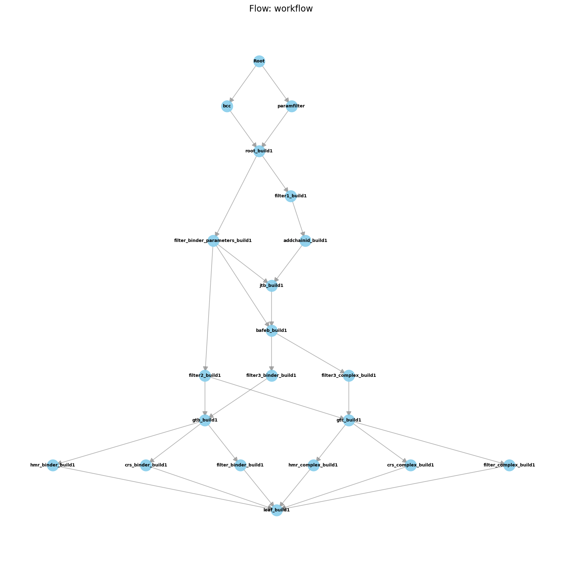
Each node in the graph is a WorkNode, while the edges represent the work dependencies between the WorkNodes and also
take the artifacts from one WorkNode to the next.
13.2.1.4. Schedulers
Schedulers decide how WorkNodes get executed, depending on the available resources. To do this, they need information about the platform they will be running on:
from amberstudio.schedulers import DefaultScheduler

scheduler = DefaultScheduler(max_cores=20, max_gpus=4, allow_gpu_oversubscription=False),
Currently, AmberStudio has three built-in schedulers:
ReferenceScheduler: Executes each WorkNode on each system, one at a time, even if they could be run in parallel. Good for debugging.
DefaultScheduler: Tries to execute each WorkNode on all available systems concurrently, if resources allow.
InterleavedScheduler: Tries to execute all ready-to-run WorkNodes on all systems, if resources allow.
13.2.1.5. Pipelines
The user-facing side of AmberStudio is typically a Pipeline. The pipeline is the context of the whole run. It groups WorkNodes, artifacts, schedulers, and other components in order to orchestrate their execution.
Below is an example for a simple pipeline that calls the build flow.
from amberstudio import Pipeline
from amberstudio.flows import FlowBuild
from amberstudio.schedulers import ReferenceScheduler

pipeline = Pipeline(
    "intro_demo",
    cwd="systems",
    scheduler=ReferenceScheduler(max_cores=1, max_gpus=1, allow_gpu_oversubscription=True),
    ignore_checkpoint=True,
)

pipeline.append_flow(FlowBuild())
print(pipeline.name)
To launch the pipeline, you would run the following:
pipeline.launch()
Note
Multiple flows can be appended to the same pipeline if their input/output artifacts match up.
13.2.2. Generating Ligand Parameters with AmberStudio
To generate ligand parameters with AmberStudio, you need to start with a PDB. AmberStudio contains Flows for ligand parameterization that use the Ligand Parameterization tools described in the Ligand Parameterization tutorials located here: Using LigandParam to Parameterize Ligands
To do this with AmberStudio, you would start with the following directory structure:
<top-dir>
    run_bcc_param.py
    binder_ejm31.pdb
The contents of run_bcc_param.py are as follows:
from pathlib import Path

from amberstudio.artifacts import ArtifactContainer, BinderLigandPDB
from amberstudio.worknodes import ParametrizeBinderBCC


def main() -> None:
    cwd = Path(__file__).resolve().parent
    ligand_pdb = cwd / "binder_ejm31.pdb"

    node = ParametrizeBinderBCC(
        "param_bcc",
        root_dir=cwd,
        resname="LIG",
        atom_type="gaff2",
        charge_model="bcc",
        charge=0,
    )

    input_artifacts = ArtifactContainer("ejm31", [BinderLigandPDB(ligand_pdb)])
    node.run(input_artifacts, cwd=cwd, sysname="ejm31")


if __name__ == "__main__":
    main()
If you look at the output WorkNode folder (param_bcc), you will see all the files from the parameterization. The files you would want are:
These would be used to build a system.
Note
In this section, we demonstrated how a single WorkNode could be run independently from a Pipeline;
however, we would rarely want to do this. If we had added this WorkNode to a Pipeline, we wouldn’t
have to specify the ArtifactContainer, and the WorkNode would run over all systems.
13.2.3. Building Systems with AmberStudio
Now, we will demonstrate building a system with AmberStudio.
<top-dir>
    run_build.py
    <ejm31>/
        binder_ejm31.mol2
        binder_ejm31.lib
        binder_ejm31.frcmod
        binder_ejm31.pdb
        target_ejm31.pdb
The input files here are:
The ligand parameter files (mol2, lib, frcmod) generated from a ligand parameterization (e.g. using the above script)
binder_ejm31.pdb is a PDB of the ligand.
target_ejm31.pdb is a PDB of the protein target.
Note
AmberStudio assumes that the coordinates of binder_ejm31.pdb correspond to a docked structure. Presently, AmberStudio does not perform docking.
from pathlib import Path
import logging

from amberstudio import Pipeline
from amberstudio.flows import FlowBuild
from amberstudio.schedulers import ReferenceScheduler


def main() -> None:
    cwd = Path(__file__).resolve().parent

    pipeline = Pipeline(
        "ejm31_build",
        cwd=cwd,
        scheduler=ReferenceScheduler(max_gpus=0),
        logging_level=logging.INFO,
        ignore_checkpoint=True,
    )

    pipeline.append_flow(
        FlowBuild(
            parametrize=False,
            skippable=False,
        )
    )
    pipeline.launch()


if __name__ == "__main__":
    main()
Note a few things about this script:
We set up a pipeline this time, which contains the build flow.
Since we already parameterized the ligands, we set parametrize to False.
This script brings you from the above files, all the way to a built parm7 and rst7 pair for both the aqueous (ligand in water) and complex configurations (ligand in protein) of the ligand.
Now let’s explore the ejm31 folder. You will see that there are many different folders that have been added. Each folder was the working directory of a separate WorkNode in the calculation.
The leaf_build folder contains the output systems.
Note
These leaf WorkNodes are called “dummy” WorkNodes because they don’t usually do anything but collect the output from a flow into a single directory. Pipelines do the same when they start, they collect all input files into a Root WorkNode.
Try opening these with VMD.
vmd python complex_ejm31.parm7 complex_ejm31.rst7
You should see the ligand bound into the protein. In the current example, HMR was applied to the system to use hydrogen-mass repartitioning. No Molecular Dynamics has been run yet.
13.2.4. Running Free-MD with AmberStudio
13.2.4.1. System Equilibration
Let’s consider that you have built a protein-ligand complex (e.g. through the system build tutorial), and you want to run free MD on that built system. The first thing needed is to run an equilibration on that system.
We will first prepare a new simulation directory to run this calculation.
<equil-dir>/
    run_equil.py
    ejm31/
        binder_ejm31.parm7
        binder_ejm31.rst7
        binderref_ejm31.rst7
        complex_ejm31.parm7
        complex_ejm31.rst7
        complexref_ejm31.rst7
You can either download this folder from here: XXX LINK XXX or generate it by copying the files from the leaf_build folder you used previously.
Note
A third option would be to append the equilibration flow in run_equil.py to the previous build pipeline script to run both one after another; however, the present tutorial will assume you are starting from a built topology.
The contents of run_equil.py are as follows.
from pathlib import Path

from amberstudio import Pipeline
from amberstudio.flows import FlowRoeRelax
from amberstudio.schedulers import ReferenceScheduler


def main() -> None:
    cwd = Path(__file__).resolve().parent

    pipeline = Pipeline(
        "ejm31_equil",
        cwd=cwd,
        scheduler=ReferenceScheduler(
            max_cores=20,
            max_gpus=1,
            allow_gpu_oversubscription=False,
        ),
        logging_level=10,
        ignore_checkpoint=True,
    )

    pipeline.append_flow(
        FlowRoeRelax(
            complex_full_restraint_mask=":1-178",
            complex_noh_restraint_mask=":1-178&!@H=",
            binder_full_restraint_mask=":179",
            binder_noh_restraint_mask=":179&!@H=",
            strong_restraint_wt=50,
            bb_restraint_mask="@CA,N,C | :1&!@H=",
            bb_restraint_wt=5,
            nstlim=120,
            nstlim_density_equilibration=120,
            skippable=True,
        )
    )

    pipeline.launch()


if __name__ == "__main__":
    main()
Warning
This will run an equilibration on a GPU. Make sure you are on an interactive GPU node prior to launching.
Note
For the purposes of this tutorial, we set nstlim=120 to keep the MD calculation short. Much longer runs are needed for actual equilibration.
Now, if things worked, you should see a short MD run complete. If you cd into the ejm31 folder, you will see many more folders, each with _roerelax (the name of the flow) appended to their names. Each of these corresponds to an MD stage that roughly corresponds to minimization -> heating -> density equilibration -> lower restraints on protein -> short free MD.
The output files are located in leaf_roerelax. You’ll note these are the mdouts, the trajectory from the last step, the topology and an equilibrated structure.
13.2.4.2. Appending Free-MD
Now, we could do the same thing as we did at the start of this tutorial: make a new directory, copy the files from leaf_roerelax, and then start a new pipeline. Instead, let’s just modify the existing pipeline to run free MD.
We have to make a few changes to our python script.
At the top of the file, add
from amberstudio.worknodes import MDParameters, MDRun
Then, between the FlowRoeRelax append and pipeline.launch(), add
filterinputcomplex = Filter(
    wnid="filterinputcomplex",
    artifact_types=(
        BaseComplexTopologyFile,
        BaseComplexStructureFile,
        BaseComplexStructureReferenceFile,
    ),
    skippable=True,
    fail_if_no_artifacts=True,
    single=True,
)
pipeline.append_node(filterinputcomplex)

extra_free_md = MDRun(
    wnid="final_complex_freemd",
    mdin_template="md",
    mdparameters=MDParameters(
        nstlim=120,
        ntpr=10,
        dt=0.004,
        gamma_ln=5.0,
        ntwx=10,
        iwrap=0,
        nscm=0,
    ),
)
pipeline.append_node(extra_free_md)
Here we first create a filter for the protein-ligand topology (that acts on leaf_roerelax) and then append an MDRun WorkNode. Again, we use a short run time for simplicity. If you look at the final_complex_freemd folder, you will see that you have a completed MD run.
13.2.5. ABFE with AmberStudio
To run an ABFE calculation with AmberStudio, the default workflow is FlowABFEProduction. This can be appended to the original equilibration flow that we used in the system builds tutorial; however, in this tutorial we will start from the end state of that tutorial.
Download the ABFE example files
Your starting folder will look like this:
<abfe-run-dir>/
    run_abfe.py
    ejm31/
        binder_ejm31.parm7
        binder_ejm31.rst7
        binderref_ejm31.rst7
        complex_ejm31.parm7
        complex_ejm31.rst7
        complexref_ejm31.rst7
    ejm42/
        binder_ejm42.parm7
        binder_ejm42.rst7
        binderref_ejm42.rst7
        complex_ejm42.parm7
        complex_ejm42.rst7
        complexref_ejm42.rst7
    jmc27/
        binder_jmc27.parm7
        binder_jmc27.rst7
        binderref_jmc27.rst7
        complex_jmc27.parm7
        complex_jmc27.rst7
        complexref_jmc27.rst7
    jmc28/
        binder_jmc28.parm7
        binder_jmc28.rst7
        binderref_jmc28.rst7
        complex_jmc28.parm7
        complex_jmc28.rst7
        complexref_jmc28.rst7
Note that we will actually be running four separate systems here all with the same pipeline.
The full contents of run_abfe.py are included below. Most are reproduced from the earlier tutorial; however, the new addition is FlowABFEProduction.
from pathlib import Path

from amberstudio import Pipeline
from amberstudio.flows import FlowABFEProduction, FlowBuild, FlowRoeRelax
from amberstudio.schedulers import ReferenceScheduler


def main() -> None:
    cwd = Path(__file__).resolve().parent

    pipeline = Pipeline(
        "abfe",
        cwd=cwd,
        scheduler=ReferenceScheduler(
            max_cores=10,
            max_gpus=1,
            allow_gpu_oversubscription=False,
        ),
        logging_level=10,
        ignore_checkpoint=True,
    )

    pipeline.append_flow(
        FlowABFEProduction(
            heating_restraint_mask=":1-290&!@H=",
            heating_restraint_wt=5,
            complex_restraint_mask=":1-290&!@H=",
            complex_restraint_wt=5,
            binder_nlambdas=3,
            complex_nlambdas=3,
            nstlim_free_binder=20,
            nstlim_free_complex=20,
            nstlim_heat=120,
            nstlim_equil1=120,
            nstlim_equil2=120,
            nstlim_trial=120,
            ntpr_trial=120,
            ntwx_trial=0,
            nmropt=True,
            numexchg_binder=5,
            numexchg_complex=5,
            start_trial_binder=1,
            end_trial_binder=1,
            start_trial_complex=1,
            end_trial_complex=1,
            lambda_max_systems=1,
            skip_analysis=True,
            skippable=True,
        )
    )

    pipeline.launch()


if __name__ == "__main__":
    main()
When you run this, you will see output that tells you that each WorkNode is executing on each of the systems independently.
FlowABFEProduction roughly performs the following steps:
Lambda annihilation: Generates lambda windows from the provided lambda schedule.
Equilibration: Equilibrates those lambda windows without replica exchange.
Production: Turns on replica exchange between lambda states.
Analysis: Runs
edgembar-amber2datsandedgembarto produce an HTML report for each ABFE calculation.
As always, the most important output is stored in the leaf node: leaf_abfeproduction.