Calculating Absolute Binding Free Energies of Tyk2 Inhibitors
Learning objectives
Learn to use AmberFlow to set up and run absolute binding free energy calculations (ABFE) for a protein-ligand system.
Relevant literature
Coming Soon!
Activities
In this Activity, you will learn how to set up and run absolute binding free energy calculations using AmberFlow, a workflow engine developed in the York Lab for automating alchemical free energy calculations with Amber.
Running ABFE Calculations with AmberFlow
In this section, we will walk through how to use AmberFlow to set up and run absolute binding free energy calculations (ABFE) for a Tyk2 inhibitor.
The files you will need are located here:
If you have not already done so, please follow the instructions in the AmberFlow documentation to install AmberFlow and set up your environment.
Warning
Currently, AmberFlow documentation is not available online. This should be updated when that changes.
Now, we will walk through the steps to get set up to run ABFE calculations with AmberFlow.
The first step is to unpack the activity files; here we will unpack them into a directory called amberflow_files:
mkdir amberflow_files
cd amberflow_files
tar -xvzf ../amberflow_files.tar.gz
In this folder, you will have a folder called starting_files. This folder contains the starting structure files for the Tyk2 protein and four ligands. The ligands are:
ejm31
ejm42
jmc27
jmc28
As you work through the activity, you will be doing certain steps. The pipeline states after each of these steps is shown in blocks below.
Initial Pipeline after Parameterization
Initial Pipeline after Building
Initial Pipeline after Equilibration
Initial Pipeline after Building
Initial Pipeline after ABFE
Parameterizing the Ligands
For the present activity, we will use the GAFF2 force field with BCC charges to parameterize the ligands. We will use AmberFlow’s connection to the ligandparam package for automated ligand parameterization.
To do this, we will start by generating a small AmberFlow script to run this parameterization. Write an initial Python file, e.g. run_parameterization.py, with the following contents:
import logging
from pathlib import Path

from amberflow.schedulers import ReferenceScheduler
from amberflow.worknodes import ParametrizeBinderBCC
from amberflow import Pipeline

home_dir = Path.cwd()
starting_files = home_dir / "tyk2"

# Define the pipeline object
pipa = Pipeline("tyk2_abfe",
              cwd=starting_files,
              scheduler=ReferenceScheduler(max_cores=10,
                                        max_gpus=1,
                                        allow_gpu_oversubscription=False),
              logging_level = logging.DEBUG,
              ignore_checkpoint=True)

# Add a worknode for the ligand parameterization.
param_node = ParametrizeBinderBCC(
wnid="bcc",
charge=0,
charge_model='bcc',
skippable=True
)
pipa.append_node(param_node)

pipa.draw()
pipa.launch()
Now this will parameterize the ligands in the tyk2 folder. You can run this script with the following command:
python run_parameterization.py
This will generate output that looks like this:
2025-10-15 11:33:49 - DEBUG - 0.0.1 Loading system jmc28
2025-10-15 11:33:49 - DEBUG - 0.0.1 Loading system ejm42
2025-10-15 11:33:49 - DEBUG - 0.0.1 Loading system jmc27
2025-10-15 11:33:49 - DEBUG - 0.0.1 Loading system ejm31
2025-10-15 11:33:49 - INFO - 0.0.1 Skipping WorkNodeDummy - Root. Status is WorkNodeStatus.COMPLETED.
2025-10-15 11:33:49 - INFO - 0.0.1 Start ParametrizeBinderBCC - bcc
2025-10-15 11:33:59 - INFO - 0.0.1 Node bcc completed on system ejm31
2025-10-15 11:34:06 - INFO - 0.0.1 Node bcc completed on system ejm42
2025-10-15 11:34:09 - INFO - 0.0.1 Node bcc completed on system jmc28
2025-10-15 11:34:10 - INFO - 0.0.1 Node bcc completed on system jmc27
Now, if you look into any of the directories within the tyk2 folder, you will see that there are now new folders present.
The first folder is Root, and is always the base folder created during any AmberFlow run. If starting with pre-parameterized ligands, you would put those in the base ligand folder and skip the parameterization step. Those files would then be copied into Root, which would be the starting point for that pipeline. In this case, if you look in Root, you will see that it is just a copy of the three pdb files that were in the tyk2 folder to start with.
The second folder is bcc, which contains the output of the ligand parameterization. There are a lot of new files, but the most important are the ones that end with *.frcmod*, *.lib*, and *.mol2*. These are the files that contain the parameters for the ligand. This folder, and the actions that it took, are an example of a WorkNode. WorkNodes are the base building blocks of AmberFlow pipelines. They take in a set of inputs, perform some action, and then generate a set of outputs. Outputs and inputs are referred to as artifacts in AmberFlow, and can be files (but can also be information such as whether the target is a protein or a nucleic acid). In this case, the binder_pdb files were the input file artifacts, and the frcmod, lib, and mol2 files were the output file artifacts.
If you explore the remaining ligand folders, you will see that they contain the same types of files. AmberFlow always runs by applying the same set of WorkNodes to each system. Other parameterization options exist, such as running a quantum calculation to generate RESP charges, or using the ABCG2 charge model. These are all available as different WorkNodes.
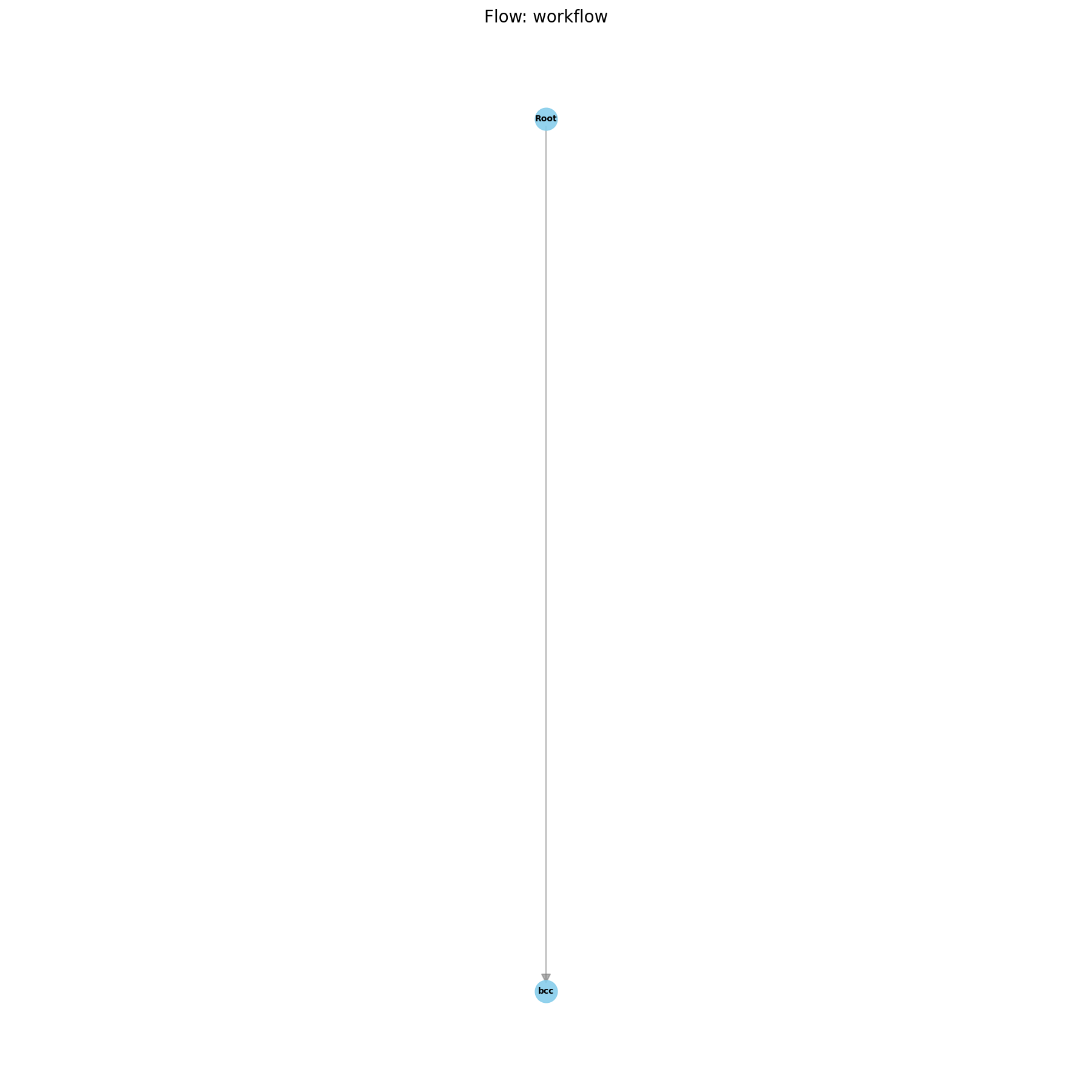
So far, our pipeline looks fairly simple, which you can see in the below figure, but will get more complicated as we move to the next steps.
Building the Systems
The next piece needed for any ABFE calculation is to build the systems. This includes solvating the protein-ligand complex, solvating the ligand alone, and generating the topology files for each of these systems. Such processes involve a number of WorkNodes, each taking a single step along this process. Here, we will use our first “Flow” to accomplish this task. Within AmberFlow, a flow is a collection of WorkNodes that are applied to each system.
To do this, we will copy the parameterization script we used above, and modify it to include a flow for building the systems. By leaving skippable=True in the parameterization worknode, we won’t redo the work if it has already been done, but will instead just automatically use the existing output artifacts.
For completeness, here is the full script, which you can save as run_abfe_build.py:
# OLD CODE
import logging
from pathlib import Path

from amberflow.schedulers import ReferenceScheduler
from amberflow.worknodes import ParametrizeBinderBCC
from amberflow import Pipeline

home_dir = Path.cwd()
starting_files = home_dir / "tyk2"

# Define the pipeline object
pipa = Pipeline("tyk2_abfe",
              cwd=starting_files,
              scheduler=ReferenceScheduler(max_cores=10,
                                        max_gpus=1,
                                        allow_gpu_oversubscription=False),
              logging_level = logging.DEBUG,
              ignore_checkpoint=True)

# Add a worknode for the ligand parameterization.
param_node = ParametrizeBinderBCC(
wnid="bcc",
charge=0,
charge_model='bcc',
skippable=True
)
pipa.append_node(param_node)
# NEW CODE
from amberflow.worknodes import Filter
from amberflow.artifacts import BinderLigandPDB
filter1 = Filter(
  wnid=f"paramfilter",
  artifact_types=(BinderLigandPDB,),
  skippable=True,
  fail_if_no_artifacts=True,
  single=True,
  in_or_out="out"
)

from amberflow.flows import FlowBuild1


# Write a flow to build the systems
build_flow = FlowBuild1(
ffpopt=False,
aq_buffer=16.0,
com_buffer=10.0
)

# append the build flow to the pipeline
pipa.append_node(filter1, pipa.root, update_leaves="none")
pipa.append_flow(build_flow)
pipa.add_edge(filter1, "root_build1")


# OLD CODE
pipa.draw()
pipa.launch()
Now here, we have appended two things to the pipeline. First, we appended a filter WorkNode. This WorkNode is used to filter the artifacts that are passed between WorkNodes. In this case, we are filtering so that the binder_pdb in the bcc WorkNode from the parameterization is used over the binder PDB in the root folder. Filters are important when you have multiple WorkNodes that generate the same type of artifact, and you want to make sure that the correct one is passed to the next WorkNode. While in general the most recent artifact is the one that should be used, there are cases where this is not true, and so filters allow (and AmberFlow requires) that you explicitly pass only the artifacts you want to the next WorkNode.
Warning
If you do not use a filter in this case, AmberFlow will raise an error and not run the pipeline. To see this behavior, you can try commenting out the filter lines and running the script again. You will see an error message indicating that there are multiple artifacts of the same type and that a filter is needed to resolve the ambiguity.
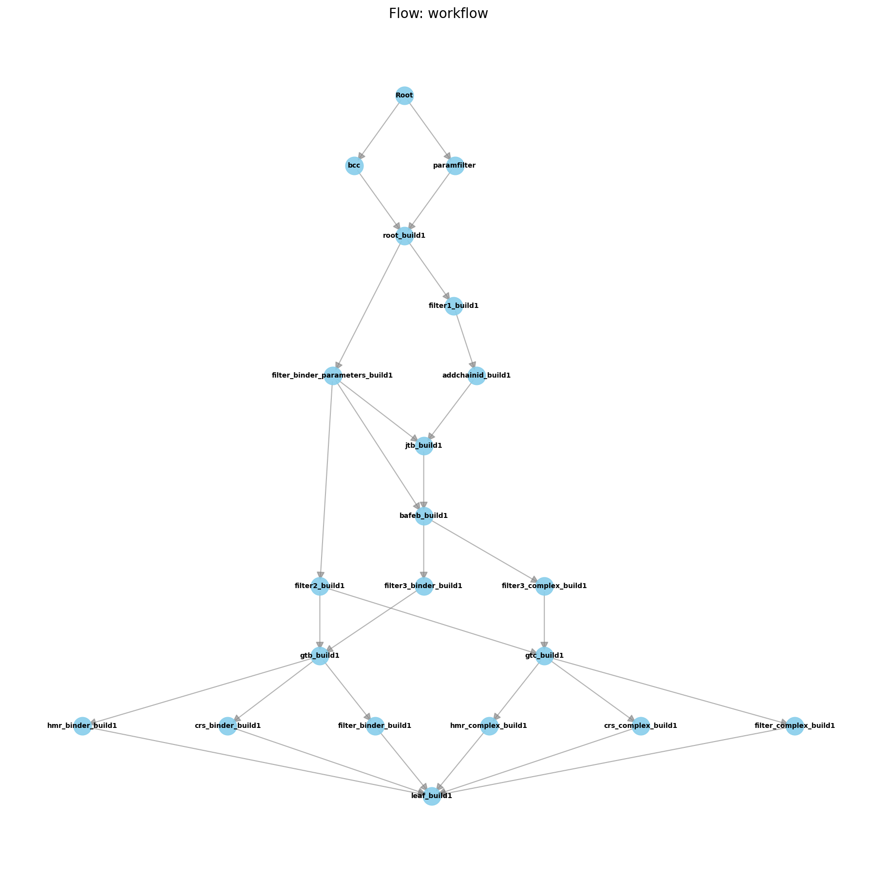
The second thing we appended was a flow, which is a collection of worknodes that are applied in sequence. You can see that the flow diagram generated by the pipa.draw() command has grown significantly. The FlowBuild1 flow contains all the worknodes needed to build the solvated protein-ligand and ligand-only systems, as well as generate the topology files for each of these systems. You’ll also see that there is quite a bit of branching in the flow. Worknodes in the pipeline happen from top to bottom, so any worknode that is below another worknode will not be run until the worknode above it has completed.
Now, if you take a look in any of the ligand folders you will see that there are now MANY new folders present. Each of these folders corresponds to a worknode in the flow. The names of the folders correspond to the wnid parameter that was used when creating the workdnode (with flows having certain defaults for wnid). The first folder in the flow will have “root” in the name (in this case, we used this above when we called “root_build1” in the add_edge command). This is the starting point for the flow, and will contain a copy of all the files that were present in the folder before the flow was run. Then, the final folder of each flow will be the leaf folder, which contains the final output files of the flow. In this case, the leaf folders are called “leaf_build1”.
If you look at this leaf folder for the ligand ejm31, you will see that it contains the following files:
binder_ejm31.parm7: The topology file for the ligand-only system.
binder_ejm31.rst7: The restart file for the ligand-only system.
binderref_ejm31.rst7: The restart file for the ligand-only system that will be used as a reference for restraints.
complex_ejm31.parm7: The topology file for the protein-ligand complex.
complex_ejm31.rst7: The restart file for the protein-ligand complex.
complexref_ejm31.rst7: The restart file for the protein-ligand complex that will be used as a reference for restraints.
If you visualize these structures for each ligand, you will see that they are all built and solvated with the same number of water molecules, and that a physiological concentration of NaCl ions have been added to each system.
Running End State Equilibrations
Warning
The remainder of this activity requires running real amber calculations which can be time consuming, and maybe not compatible with local resources depending on your current environment. If you want to run these calculations on a different system, copy the entire directory structure that you have run thus far to that system and then run the next steps there. AmberFlow, Amber, and FE-Toolkit must be installed on that system.
Note
When running on another system, you may want to modify the scheduler parameters in the pipeline definition to match the resources available on that system. Currently, this script uses ReferenceScheduler which runs 1 system at a time, but on systems with multiple GPUs, you may want to use DefaultScheduler instead (and then modify max_cores and max_gpus accordingly). Also, usually allow_gpu_oversubscription should be set to True on systems with multiple GPUs as this will better use the available resources.
from amberflow.schedulers import DefaultScheduler

pipa = Pipeline("tyk2_abfe",
              cwd=starting_files,
              scheduler=DefaultScheduler(max_cores=40,
                                        max_gpus=4,
                                        allow_gpu_oversubscription=True),
              logging_level = logging.DEBUG,
              ignore_checkpoint=True)
The next step in the ABFE calculation is to equilibrate the systems. Roughly, this involves a number of minimization, heating, and equilibration steps. AmberFlow provides a flow, FlowRoeRelax1, that contains all the WorkNodes needed to perform these steps:
Minimize the system with restraints on the protein + ligand
Minimize the system without restraints
Fix Clashes
Heat the system from 0K to 300K with restraints on the protein + ligand
Equilibrate the density in a series of short simulations with restraints on the protein + ligand
Equilibrate the system at 300K and 1 atm with restraints on the protein
Slowly reduce the restraints on the protein and ligand
Equilibrate the system at 300K and 1 atm without restraints
To add this flow to the pipeline, we will copy the script from above and modify it to include this new flow. Save this as run_abfe_equil.py:
# OLD CODE
import logging
from pathlib import Path

from amberflow.schedulers import ReferenceScheduler
from amberflow.worknodes import ParametrizeBinderBCC
from amberflow import Pipeline

home_dir = Path.cwd()
starting_files = home_dir / "tyk2"

# Define the pipeline object
pipa = Pipeline("tyk2_abfe",
              cwd=starting_files,
              scheduler=ReferenceScheduler(max_cores=10,
                                        max_gpus=1,
                                        allow_gpu_oversubscription=False),
              logging_level = logging.DEBUG,
              ignore_checkpoint=True)

# Add a worknode for the ligand parameterization.
param_node = ParametrizeBinderBCC(
wnid="bcc",
charge=0,
charge_model='bcc',
skippable=True
)
pipa.append_node(param_node)

from amberflow.worknodes import Filter
from amberflow.artifacts import BinderLigandPDB
filter1 = Filter(
  wnid=f"paramfilter",
  artifact_types=(BinderLigandPDB,),
  skippable=True,
  fail_if_no_artifacts=True,
  single=True,
  in_or_out="out"
)

from amberflow.flows import FlowBuild1


# Write a flow to build the systems
build_flow = FlowBuild1(
ffpopt=False,
aq_buffer=16.0,
com_buffer=10.0
)

# append the build flow to the pipeline
pipa.append_node(filter1, pipa.root, update_leaves="none")
pipa.append_flow(build_flow)
pipa.add_edge(filter1, "root_build1")

# New Code

from amberflow.flows import FlowRoeRelax1

relax_flow = FlowRoeRelax1(
  complex_full_restraint_mask=":1-289",
  complex_noh_restraint_mask=":1-289&!@H=",
  binder_full_restraint_mask=":1",
  binder_noh_restraint_mask=":1&!@H=",
  strong_restraint_wt=50,
  bb_restraint_mask="@CA,N,C | :1&!@H=",
  bb_restraint_wt=5,
  complex_free_restraint_mask=None,
  complex_free_restraint_wt=5,
  nstlim=1000000,
  nstlim_density_equilibration=20000,
  skippable=True,
)

pipa.append_flow(relax_flow)


# OLD CODE
pipa.draw()
pipa.launch()
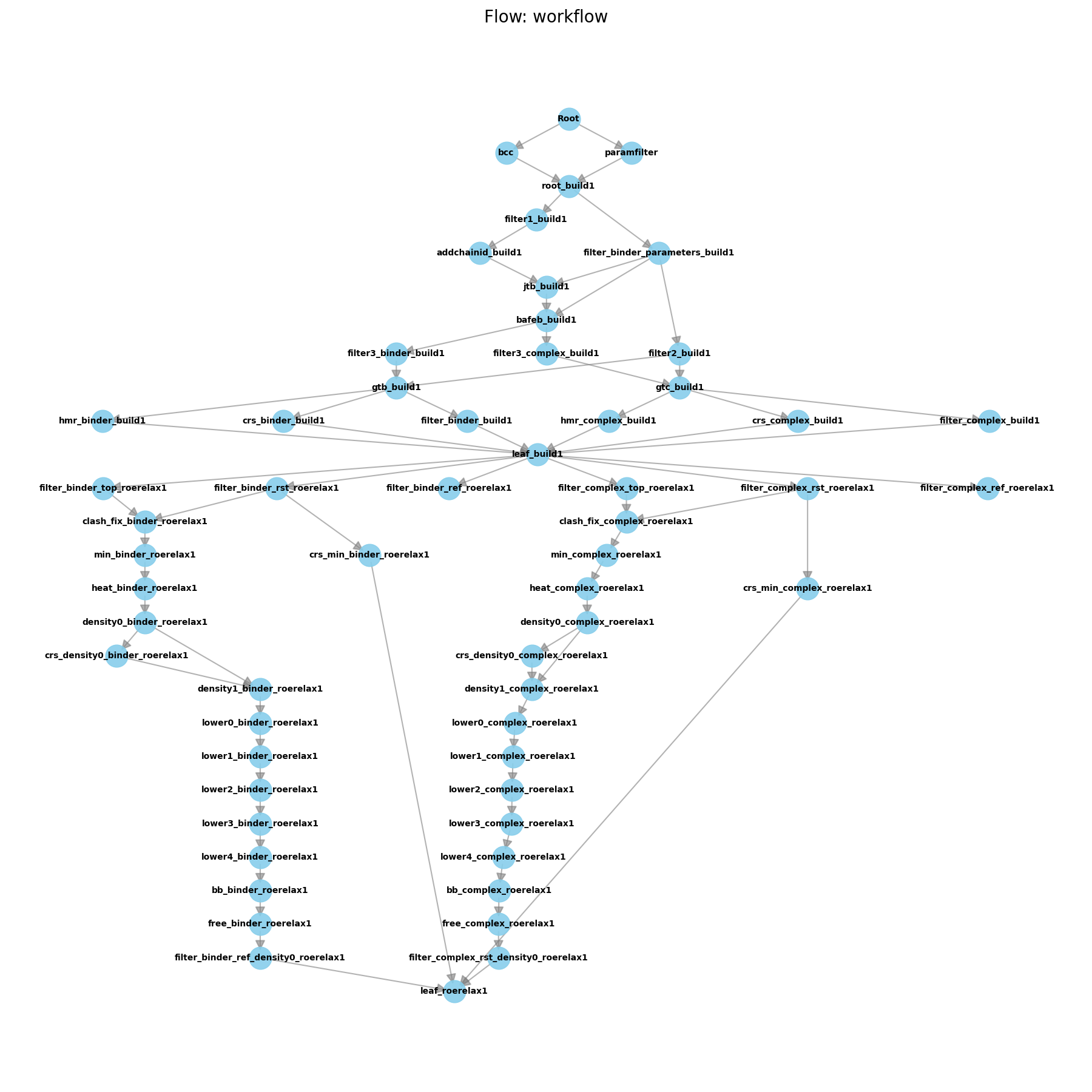
Here, we have appended the FlowRoeRelax1 flow to the pipeline. This flow contains all the worknodes needed to perform the equilibration steps outlined above. Note here that we have specified a number of parameters for the flow, such as the restraint masks and weights. These parameters are important for ensuring that the equilibration is performed correctly. You will need to modify these parameters based on your system. The parameters used here are appropriate for the Tyk2 system, which has 288 residues and a single ligand residue (hence 1-289) in the complex restraint mask (which includes the ligand as residue 1).
Now if you run this script, you will see that the flow diagram has grown even more, with the new flow connecting to the leaf folder of the previous flow. This is because the output artifacts of the previous flow are the input artifacts for this flow. The leaf folder of this new flow is called “leaf_roerelax1”, and contains the final equilibrated structures for each system.
If you look in this folder for the ligand ejm31, you will see that it contains the following files:
binder_ejm31.mdout: The amber mdout file for the ligand-only system.
binder_ejm31.parm7: The topology file for the ligand-only system.
binder_ejm31.rst7: The restart file for the ligand-only system.
binderref_ejm31.rst7: The restart file for the ligand-only system that will be used as a reference for restraints.
binder_ejm31.nc: The amber trajectory file for the ligand-only system.
complex_ejm31.mdout: The amber mdout file for the protein-ligand complex.
complex_ejm31.parm7: The topology file for the protein-ligand complex.
complex_ejm31.rst7: The restart file for the protein-ligand complex.
complexref_ejm31.rst7: The restart file for the protein-ligand complex that will be used as a reference for restraints.
complex_ejm31.nc: The amber trajectory file for the protein-ligand complex.
node.log: The AmberFlow log file for the flow.
Note - these are all the files that would be necessary to run ABFE calculations. However, we are not quite ready to run ABFE yet. There is one more piece we need to add to the pipeline before we can run ABFE calculations, which is to determine the Boresch restraints that will be used to restrain the ligand in the binding site during the ABFE calculations. This will be covered in the next section.
Determining Boresch Restraints Using AmberFlow
Now we are almost ready for ABFE! The last piece we need before running actual ABFE calculatioons is to determine the Boresch restraints that will be used to restrain the ligand in the binding site when its interactions are decoupled from the protein during Hamiltonian replica exchange simulations. As you might surmise by this point, AmberFlow has a WorkNode that can do this for us!
# OLD CODE
import logging
from pathlib import Path
from amberflow.schedulers import ReferenceScheduler
from amberflow.worknodes import ParametrizeBinderBCC
from amberflow import Pipeline
home_dir = Path.cwd()
starting_files = home_dir / "tyk2"
# Define the pipeline object
pipa = Pipeline("tyk2_abfe",
cwd=starting_files,
scheduler=ReferenceScheduler(max_cores=10,
max_gpus=1,
allow_gpu_oversubscription=False),
logging_level = logging.DEBUG,
ignore_checkpoint=True)
# Add a worknode for the ligand parameterization.
param_node = ParametrizeBinderBCC(
wnid="bcc",
charge=0,
charge_model='bcc',
skippable=True
)
pipa.append_node(param_node)
from amberflow.worknodes import Filter
from amberflow.artifacts import BinderLigandPDB
filter1 = Filter(
wnid=f"paramfilter",
artifact_types=(BinderLigandPDB,),
skippable=True,
fail_if_no_artifacts=True,
single=True,
in_or_out="out"
)
from amberflow.flows import FlowBuild1
# Write a flow to build the systems
build_flow = FlowBuild1(
ffpopt=False,
aq_buffer=16.0,
com_buffer=10.0
)
# append the build flow to the pipeline
pipa.append_node(filter1, pipa.root, update_leaves="none")
pipa.append_flow(build_flow)
pipa.add_edge(filter1, "root_build1")
from amberflow.flows import FlowRoeRelax1
relax_flow = FlowRoeRelax1(
complex_full_restraint_mask=":1-289",
complex_noh_restraint_mask=":1-289&!@H=",
binder_full_restraint_mask=":1",
binder_noh_restraint_mask=":1&!@H=",
strong_restraint_wt=50,
bb_restraint_mask="@CA,N,C | :1&!@H=",
bb_restraint_wt=5,
complex_free_restraint_mask=None,
complex_free_restraint_wt=5,
nstlim=1000000,
nstlim_density_equilibration=20000,
skippable=True,
)
pipa.append_flow(relax_flow)
# New Code
from amberflow.worknodes import GetBoresch
boresch_complex = GetBoresch(wnid="boresch_complex", skippable=True)
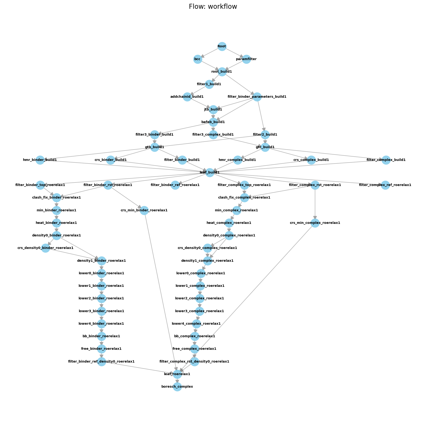
pipa.append_node(boresch_complex, update_leaves="add")
# OLD CODE
pipa.draw()
pipa.launch()
This worknode will analyze the equilibrated complex structure and determine the optimal set of Boresch restraints to use for ABFE calculations. These restraints will then be used in the ABFE calculations to restrain the ligand in the binding site. If you look into the boresch_complex folder within ejm_31, you will see the output of this command after running it.
The file produced looks like this:
&rst iat=1489,15,0
r1=0.00000,r2=4.46147,r3=4.46147,r4=999.000,rk2=14.62, rk3=14.62/
&rst iat=1477,1489,15,0
  r1=-180.00000,r2=84.48356,r3=84.48356,r4=180.000,rk2=54.14, rk3=54.14/
&rst iat=1489,15,14,0
  r1=-180.00000,r2=66.83900,r3=66.83900,r4=180.000,rk2=37.54, rk3=37.54/
&rst iat=1490,1477,1489,15,0
  r1=-180.00000,r2=14.62579,r3=14.62579,r4=180.000,rk2=42.50, rk3=42.50/
&rst iat=1477,1489,15,14,0
  r1=-180.00000,r2=28.80971,r3=28.80971,r4=180.000,rk2=64.34, rk3=64.34/
&rst iat=1489,15,14,16,0
  r1=-180.00000,r2=-138.45151,r3=-138.45151,r4=180.000,rk2=52.87, rk3=52.87/
Running the ABFE Flow within AmberFlow
Note
This next section deals with running ABFE calculations. ABFE calculations are computationally expensive, and you may want to run this on supercomputing resources if you have access to them. These runs may take up to 48 hours per ligand on a single GPU, so plan accordingly. If you do not have access to supercomputing resources, you can still run this activity, but you may want to run far fewer steps and reduce the number of lambda windows. Such changes will make your results inaccurate, but will allow you to see how the pipeline works without needing to wait for days.
In this section of the activity, we will add the final flow to the pipeline, which is the FlowABFE7 flow. This flow contains all the worknodes needed to perform ABFE calculations using Hamiltonian replica exchange with Alchemically Enhanced Sampling. This flow will use the equilibrated structures from the previous flow, as well as the Boresch restraints determined in the previous section.
The rough steps involved in this flow are:
Annihilated the ligand in the complex and ligand-only systems using a series of lambda windows.
Reinitialize and Reheat the system from 100 K to 300 K
Equilibrate the Lambda Windows
Run Production Hamiltonian Replica Exchange Simulations
Analyze the results using FE-Toolkit and EdgeMBAR to determine the free energy of binding.
To add this flow to the pipeline, we will copy the script from above and modify it to include this new flow. Save this as run_abfe.py:
# OLD CODE
import logging
from pathlib import Path

from amberflow.schedulers import ReferenceScheduler
from amberflow.worknodes import ParametrizeBinderBCC
from amberflow import Pipeline

home_dir = Path.cwd()
starting_files = home_dir / "tyk2"

# Define the pipeline object
pipa = Pipeline("tyk2_abfe",
              cwd=starting_files,
              scheduler=ReferenceScheduler(max_cores=10,
                                        max_gpus=1,
                                        allow_gpu_oversubscription=False),
              logging_level = logging.DEBUG,
              ignore_checkpoint=True)

# Add a worknode for the ligand parameterization.
param_node = ParametrizeBinderBCC(
wnid="bcc",
charge=0,
charge_model='bcc',
skippable=True
)
pipa.append_node(param_node)

from amberflow.worknodes import Filter
from amberflow.artifacts import BinderLigandPDB
filter1 = Filter(
  wnid=f"paramfilter",
  artifact_types=(BinderLigandPDB,),
  skippable=True,
  fail_if_no_artifacts=True,
  single=True,
  in_or_out="out"
)

from amberflow.flows import FlowBuild1


# Write a flow to build the systems
build_flow = FlowBuild1(
ffpopt=False,
aq_buffer=16.0,
com_buffer=10.0
)

# append the build flow to the pipeline
pipa.append_node(filter1, pipa.root, update_leaves="none")
pipa.append_flow(build_flow)
pipa.add_edge(filter1, "root_build1")


from amberflow.flows import FlowRoeRelax1

relax_flow = FlowRoeRelax1(
  complex_full_restraint_mask=":1-289",
  complex_noh_restraint_mask=":1-289&!@H=",
  binder_full_restraint_mask=":1",
  binder_noh_restraint_mask=":1&!@H=",
  strong_restraint_wt=50,
  bb_restraint_mask="@CA,N,C | :1&!@H=",
  bb_restraint_wt=5,
  complex_free_restraint_mask=None,
  complex_free_restraint_wt=5,
  nstlim=1000000,
  nstlim_density_equilibration=20000,
  skippable=True,
)

pipa.append_flow(relax_flow)


from amberflow.worknodes import GetBoresch
boresch_complex = GetBoresch(wnid="boresch_complex", skippable=True)
pipa.append_node(boresch_complex, update_leaves="add")


# New Code

from amberflow.flows import FlowABFE7

binder_windows = [
0.00000000, 0.13098000, 0.21201000, 0.26401000, 0.30636000, 0.34433000,
0.37938000, 0.41236000, 0.44434000, 0.47551000, 0.50621000, 0.53668000,
0.56698000, 0.59718000, 0.62685000, 0.65568000, 0.68242000, 0.70731000,
0.73179000, 0.75770000, 0.78666000, 0.82089000, 0.86930000, 1.00000000,
]

complex_windows = [
0.00000000, 0.13102000, 0.21119000, 0.26280000, 0.30471000, 0.34202000,
0.37647000, 0.40898000, 0.44048000, 0.47140000, 0.50177000, 0.53204000,
0.56183000, 0.59113000, 0.62058000, 0.65039000, 0.68020000, 0.70877000,
0.73602000, 0.76324000, 0.79211000, 0.82503000, 0.86947000, 1.00000000,
]


abfe_flow = FlowABFE7(
    binder_windows=binder_windows,
    complex_windows=complex_windows,
    heating_restraint_mask=":1-289&!@H=",
    heating_restraint_wt=5,
    complex_rmsd_mask1=":1 & !@H=",
    complex_rmsd_strength1_heat=0,
    complex_rmsd_strength1_equil1=0,
    complex_rmsd_strength1_equil2=0,
    complex_rmsd_strength1_trial_equil=0,
    complex_rmsd_strength1_trial=0,
    complex_rmsd_ti1=2,
    complex_rmsd_mask2="@CA ",
    complex_rmsd_strength2_heat=0,
    complex_rmsd_strength2_equil1=0,
    complex_rmsd_strength2_equil2=0,
    complex_rmsd_strength2_trial_equil=0,
    complex_rmsd_strength2_trial=0,
    complex_rmsd_ti2=3,
    binder_rmsd_mask=":1 & !@H=",
    binder_rmsd_strength_heat=0,
    binder_rmsd_strength_equil1=0,
    binder_rmsd_strength_equil2=0,
    binder_rmsd_strength_trial_equil=0,
    binder_rmsd_strength_trial=0,
    binder_rmsd_ti=2,
    complex_rmsd_type=0,
    binder_rmsd_type=0,
    nstlim_heat=100000,
    nstlim_equil1=50000,
    nstlim_equil2=250000,
    nstlim_trial_equil=250000,
    nstlim_trial=100,
    bar_intervall=100,
    ntwx_trial=1250,
    numexchg=12500,
    nmropt=True,
    start_trial=1,
    end_trial=1,
    skippable=True,
    skip_analysis=False,
    max_systems_binder = 1,
    max_systems_complex = 1,
)

pipa.append_flow(abfe_flow)


# OLD CODE
pipa.draw()
pipa.launch()
Note that in the above script, we have specified a wide-range of parameters for the ABFE calculations, most of which are left at their default values. Many of these are related to features that we won’t be using for this activity, such as RMSD and lambda-dependent RMSD restraints (set to 0 above); however, many of the other parameters have significant impacts on calculated results.
In general, anything marked nstlim_XXX is the number of steps to run for that phase of the calculation. The values used above are appropriate for a production ABFE calculation, but you may want to reduce these values if you are running on a local machine and want to see results quickly. The total production length in steps is determined by bar_intervall*numexchg.
start_trial and end_trial determine how many trials to run. Each trial is an independent repeat of an equilibration and production run. More trials will give better statistics, but will also take longer to run. For a production calculation, you will want to run at least 3 trials, but for testing purposes, you can set both of these to 1 to just run a single trial.
max_systems_binder and max_systems_complex determine how many systems to run in parallel. This is useful if you have multiple GPUs available, as you can run multiple systems at once to better utilize the available resources. However, if you are running on a single GPU, you will want to set these to 1 to avoid oversubscribing the GPU.
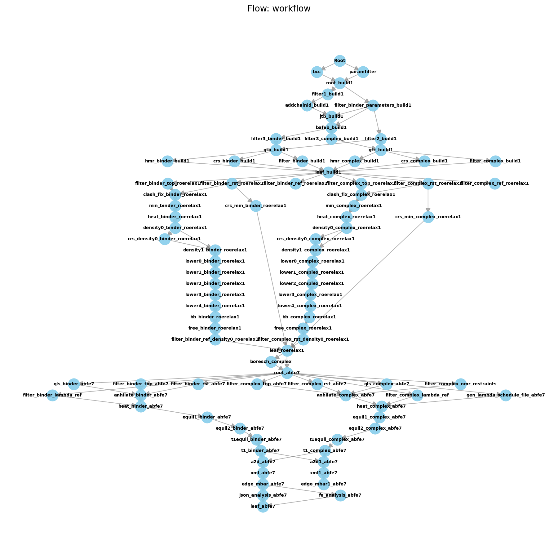
As you can see from the flow diagram, the pipeline is quite large!
Analyzing the Results
Now, the experimental binding free energies for these ligands are known. You can compare your calculated results to the experimental values to see how well the calculations performed. The experimental values are as follows:
jmc27 : -11.28 kcal/mol
jmc28 : -10.98 kcal/mol
ejm31 : -9.56 kcal/mol
ejm42 : -9.78 kcal/mol
After running the ABFE flow, you will see that in each ligand folder there is now a folder called “leaf_abfe7”. This folder contains the summary output files for the ABFE calculations. There are two main files of interest:
fe_data.csv: This file contains the free energy values summarized for all four ligands (if you ran them as a single flow). This file contains the calculated binding free energy for each ligand, as well as the associated error estimates.
edge_{ligand}.html: This file contains a detailed analysis of the free energy calculations for each ligand. It includes plots of the dU/dlambda profile, as well as other useful information about the calculations.
Note
Each ligand’s HTML file is located in that ligand’s leaf_abfe7 folder, whereas the fe_data.csv file contains information about all ligands.
For more information on the HTML files used for analysis, please check out the relevant activity.