Calculating Relative Binding Free Energies of Tyk2 Inhibitors
Learning objectives
Learn to use FE-Workflow to set up and run relative binding free energy calculations.
Activities
Warning
It is planned that FE-WORKFLOW will be replaced by AmberFlow in the near future. This activity is being written in the meantime to help users get started with RBFE calculations with Amber; however, it will be replaced once RBFE functionality is added to AmberFlow.
In this Activity, you will learn how to set up and run relative binding free energy calculations using FE-WORKFLOW, a workflow engine developed in the York Lab for automating alchemical free energy calculations with Amber.
        flowchart LR

    Mol2In[Ligand Mol2 Charges]
    LibIn[Ligand Lib File]
    FRCIn[Ligand FRCmod File]
    PDBIn[Docked PDB]
    inputIn["input_file"]

    setup_fe[bash setup_fe.sh]

    built_out_complex[Built Complex System]
    built_out_aquous[Built Aqueous System]

    run_trials[Run Trial Slurm Jobs]

    mdout_complex[MD Output Complex]
    mdout_aquous[MD Output Aqueous]
    remlog_complex[REMLog Complex]
    remlog_aquous[REMLog Aqueous]

    Amber2Dats[Amber2Dats]

    XMLOuts[XML Outputs]

    DiscoverEdges[DiscoverEdges]
    PythonOuts[Python Outputs]
    HTMLOuts[HTML]
    WriteGraph[WriteGraph]
    GraphOuts[Graph Output HTML]


    Mol2In --> setup_fe
    LibIn --> setup_fe
    FRCIn --> setup_fe
    PDBIn --> setup_fe
    inputIn --> setup_fe
    setup_fe --> built_out_complex
    setup_fe --> built_out_aquous
    built_out_complex --> run_trials
    built_out_aquous --> run_trials

    run_trials --> mdout_complex
    run_trials --> mdout_aquous
    run_trials --> remlog_complex
    run_trials --> remlog_aquous

    mdout_complex --> Amber2Dats
    mdout_aquous --> Amber2Dats
    remlog_complex --> Amber2Dats
    remlog_aquous --> Amber2Dats

    Amber2Dats --> XMLOuts
    XMLOuts --> DiscoverEdges
    DiscoverEdges --> PythonOuts
    DiscoverEdges --> WriteGraph
    PythonOuts --> HTMLOuts
    HTMLOuts --> GraphOuts
    WriteGraph --> GraphOuts

    click Mol2In "#getting-structures-and-parameters"
    click LibIn "#getting-structures-and-parameters"
    click FRCIn "#getting-structures-and-parameters"
    click PDBIn "#getting-structures-and-parameters"

    click inputIn "#preparing-the-simulation-directory"
    click setup_fe "#running-fe-workflow"

    click built_out_complex "#examining-the-outputs-of-the-build"
    click built_out_aquous "#examining-the-outputs-of-the-build"
    click run_trials "#submitting-jobs-to-the-cluster"
    click mdout_complex "#analyzing-results"
    click mdout_aquous "#analyzing-results"
    click remlog_complex "#analyzing-results"
    click remlog_aquous "#analyzing-results"
    click GraphOuts "#analyzing-results"
    click Amber2Dats "#analyzing-results"
    click XMLOuts "#analyzing-results"
    click DiscoverEdges "#analyzing-results"
    click PythonOuts "#analyzing-results"
    click HTMLOuts "#analyzing-results"
Getting Started
In this activity, we will be using the FE-WORKFLOW package from the York Group to set up and run relative binding free energy calculations (RBFE) of Tyk2 inhibitors.
To install FE-WORKFLOW, please download it from our GitLab:
git clone git@gitlab.com:RutgersLBSR/FE-Workflow.git
To install it, you need to proceed differently depending on whether you installed fe-toolkit using pip.
If you installed fe-toolkit using pip, you can install FE-WORKFLOW
source <amber installation path>/amber.sh
export PATH=<fe-toolkit installation path>/local/bin:$PATH
export PYTHONPATH=<fe-toolkit installation path>/local/lib/python3.11/site-packages:${PYTHONPATH}
export PATH=$PATH:<FE-Workflow path>/bin
If you installed fe-toolkit from source, you can install FE-WORKFLOW using the following commands:
export BACKUP_PATH=$PATH
export BACKUP_PYTHONPATH=${PYTHONPATH}
source <amber installation path>/amber.sh
export PATH=$BACKUP_PATH:$PATH
export PYTHONPATH=${BACKUP_PYTHONPATH}:$PYTHONPATH
export PATH=$PATH:<FE-Workflow path>/bin
Then, once you have done either of these, you run the following command to install FE-WORKFLOW:
makesetup_fe.sh
This should create the executable setup_fe in your PATH. This is what will be used to set up and run the RBFE calculations.
System Information
In this activity, we will be calculating the relative binding free energies of a series of Tyk2 inhibitors.
These inhibitors are the same as will be covered in the Absolute Binding Free Energy activity for Tyk2, which can be found here: Calculating Absolute Binding Free Energies of Tyk2 Inhibitors.
These are:
ejm31
ejm42
jmc27
jmc28
Getting Structures and Parameters
To get started, download the following archive which contains RESP-parameterized ligands and prepared protein-ligand complexes for the Tyk2 inhibitors:
To download the files Download Tar
Once you have downloaded the archive, extract it to a working directory where you will be running the activity.
tar -xvf tyk2_feworkflow_tutorial.tar.gz
cd tyk2_feworkflow_tutorial
In this folder, you should see the following files and directories:
parameters/: Directory containing RESP-parameterized ligands. docked_complexes: Directory containing prepared protein-ligand complexes.
Note
Parameters were generated using the protocol outlined in our Force Field Parameterization activity, which can be found here: Using LigandParam to Parameterize Ligands.
Preparing the Simulation Directory
To first set up the simulation directory for FE-WORKFLOW, we will make a working directory and copy over the necessary files.
mkdir working_dir
cd working_dir
mkdir -p initial/tyk2
cp ../parameters/* initial/tyk2/
cp ../docked_complexes/* initial/tyk2/
Next, we will create an input file for FE-WORKFLOW. This file contains all the necessary information for setting up and running the RBFE calculations.
Below, we’ve provided a sample input file which you can copy and paste into a file named input in your working directory.
#######################################################################
# 1. NAME OF SYSTEM, INPUT STRUCTURES, and TYPE OF CALCULATION
#######################################################################
# Directory that contains within it a subdirectory names "system"
# containing initial structure/parameter files.
# For example, a single folder "initial" may contain multiple
# subdirectories containing initial files for different systems
path_to_input=initial


# Subdirectory containing initial structure/parameter files
# of "system"
# For example,
#system=smallMols
system=tyk2


# setupmode determines the calculation.
# setupmode=0 --> regular TI
# setupmode=1 --> end-point ACES
# setupmode=2 --> TI from end-point ACES.
# currenty, only setupmode=0 is implemented.
setupmode=0

# ticalc determines the nature of TI calculation.
# ticalc=rbfe --> relative binding free energy
# ticalc=rsfe --> relative solvation free energy
# ticalc=asfe --> absolute solvation free energy
ticalc=rbfe

# stage controls the action of the script
# stage=setup 		--> setup of TI  simulations
# stage=analysis 	--> analysis of TI simulations using FE-ToolKit
stage=setup


# List of desired transformations or edges
# For example, RBFE or RSFE calculations should have a list
# in which each entry consists of two molnames separated by the
# character "~". Initial structure/parameter files of these
# molnames should be provided in /
# For RBFE calculations, the PDB file of protein-ligand complex
# and mol2,lib,frcmod files of ligand are expected.
# For RSFE calculations, mol2,lib,frcmod files of ligand are expected.
# example,
# translist=(1h1q~1h1r 1h1q~1h1s)
#
# For ASFE calculations, "translist" should contain a list of
# molnames.
# mol2,lib,frcmod files of these molnames are expected in
# /
# example,
#translist=(1h1q~1h1r 1h1r~1h1s 1h1s~1oiu 1oiu~1h1q 1h1r~1oiu 1h1s~1h1q)
translist=(jmc_23~ejm_55 jmc_23~ejm_44 ejm_44~ejm_55)
#######################################################################


#######################################################################
# 2. ATOM MAPPING
#######################################################################
#
# mapmethod determines the algorithm using which cc and sc regions
# will be determined.
# mapmethod=0 --> MCSS
# mapmethod=1 --> MCSS-E
# mapmethod=2 --> MCSS-E2
mapmethod=2

# mapinspect determines if there is need of manual inspection of the
# atom maps
# mapinspect=0 --> no-inspection. generate the atom maps using
# algorithm specified by "mapmethod", and then proceed to generate
# file infrastructure
# mapinspect=1 --> manual inspection. stop after generating the
# atom maps.
# mapinspect=2 --> resume generation of file infrastructure assuming
# map inspection has been completed.
# mapinspect=2 expects necessary atom map files to be present in the "setup" folder
mapinspect=0


# mapnetwork determines whether network-wide consistent cc and sc regions
# will be generated.
# mapnetwork=true ensures that in a given network of transformations, cc and sc
# regions of each ligand is identical in every transformation in which is participates
mapnetwork=true

#######################################################################

#######################################################################
# 3. MD BOX BUILDING
#######################################################################
#
# boxbuild determines if and how MD boxes will be built
# "skip" 	--> skip box building
# 0      	--> for RBFE calculations, do not build boxes for "complex" state,
#		    only for "aqueous" state.
# 1 		--> build boxes for both "complex" and "aqueous" states
# 		    for RSFE and ASFE calculations, boxbuild=0 and boxbuild=1 are
#		    identical.
# 2 		--> build boxes for both "complex" and "aqueous" states with same
#		    number of water and ions
boxbuild=2
boxbufcom=16                    # MD box buffer for "complex" states
boxbufaq=20                     # MD box buffer for "aqueous" states
ionconc=0.15                    # Ion concentration in MD box
pff=ff19SB                      # Protein force field
lff=gaff2                       # Ligand forcefield
wm=tip4pew                      # Water model
mdboxshape=oct                # Shape of MD box
#######################################################################


#######################################################################
# 4. GENERAL SETTINGS OF TI SIMULATIONS
#######################################################################
#
nlambda=24                      # number of lambda windows
lamschedule=yes
lams=(0.00000000 0.04347826 0.08695652 0.13043478 0.17391304 0.21739130 0.26086957 0.30434783 0.34782609 0.39130435 0.43478261 0.47826087 0.52173913 0.56521739 0.60869565 0.65217391 0.69565217 0.73913043 0.78260870 0.82608696 0.86956522 0.91304348 0.95652174 1.00000000)
protocol=unified                # unified protocol for TI

ntrials=3                       # Number of independent trials

cutoff=10                       # non-bonded cutoff
repex=true
nstlimti=5                     # length of TI simulations
numexchgti=300000               # number of exchanges in replica exchange TI simulations. if repex=true
hmr=true
notrajectory=true               # when true, no output trajectories are generated
scalpha=0.5                     # scalpha
scbeta=1.0                      # scbeta
gti_add_sc=25
gti_scale_beta=1                # gti_scale_beta
gti_cut=1                       # gti_cut
gti_cut_sc_on=8                 # gti_cut_sc_on
gti_cut_sc_off=10               # gti_cut_sc_off
gti_lam_sch=1                   # gti_lam_sch
gti_ele_sc=1                    # gti_ele_sc
gti_vdw_sc=1                    # gti_vdw_sc
gti_cut_sc=2                    # gti_cut_sc
gti_ele_exp=2                   # gti_ele_exp
gti_vdw_exp=2                   # gti_vdw_exp

# twostate determines the protocol to be used for equilibration of protein-ligand complex systems.
# twostate=false directs script to setup the equilibration file infrastructure
# in an "1-state" way in which for a given transformation P:A --> P:B, only the P:A structure is
# considered and the ligand B is superimposed on ligand A.
# twostate=true directs script to setup the equilibration file infrastructure
# in a "2-state" way in which for a given transformation P:A --> P:B, both P:A and P:B structures
# considered and represents the two end states.
twostate=true
bidirection_com=false
bidirection_aq=false

equil_type=2
ntwx=0
ntwx_ep=1250
ntwr=1250
ntpr=125

#######################################################################


#######################################################################
# 5. SETTINGS RELATED TO JOB SUBMISSION
#######################################################################
#
# job submission related
partition=gh      # name of specific partition on HPC. Use "null" is not relevant
nnodes=1                        # number of nodes to be used for each transformation
ngpus=1                         # number of gpus/node to be used for each transformation
wallclock=0-48:00:00            # wallclock for individual jobs
source_header="/home1/10162/piskuliche/load_flow_auto.sh"
#######################################################################

#######################################################################
# 6. ANALYSIS
#######################################################################
#
# path to production runs. default path_to_input="system"/"protocol"/run
# exptdatafile is an optional text file containing experimental free energies.
# exptdatafile can be set to "skip" or if provided, should be a file containing 2 columns.
# col 1 should be ligand name (identical to ligand name in translist) and col2 should be
# relative experimental free energy
#
path_to_data=tyk2/unified/run
exptdatafile=skip
bar=true
ccc=true
ccc_ddG=true
start=0.0
stop=100.0
check_convergence=true
showallcycles=true
#######################################################################
Below we will go through some of the key sections of this input file.
Note
The sample input file is intended to be a good starting point for the TYK2 example, not a universal set of optimal parameters. When adapting this workflow to a new system, the settings that most often need attention are the atom mapping, the lambda schedule, the number of windows, the amount of sampling per window, and any protein or ligand-specific preparation choices.
- [NAME OF SYSTEM, INPUT STRUCTURES, and TYPE OF CALCULATION]: This section specifies details about the folder structure, how you want to run the calculations, and the type of calculation.
path_to_input: The path to the input files for the system being studied. This is relative to the working directory where you are running FE-WORKFLOW.
system: The name of the system being studied. This controls the naming of the build directory, and the location within path_to_input where it expects structures and parameters to be located.
setupmode: Only 0 is currently supported.
ticalc: Specifies the type of calculation. For RBFE calculations, this should be set to rbfe.
stage: setup. This specifies that we are in the setup stage of the calculation. You can later change this to analysis to run the analysis stage.
translist: A list of ligand transformations to be performed. Each transformation is specified as a pair of ligand names separated by a ~. These names should match the names of the ligands in the input files.
[ATOM MAPPING]: This section specifies how atoms in the ligands are mapped during the transformations.
- mapmethod: The method used for atom mapping. All three methods use maximum common substructure methods to identify the common atoms between the two ligands. It is recommended to use MCSS-E2 for best results.
0: MCSS
1: MCSS-E
2: MCSS-E2
mapinspect: Whether to proceed with the whole build, or to stop after the atom mapping. Set to 0 to map and build, 1 to only map, and 2 to resume generation after inspecting the mapping.
mapnetwork: Ensures that for a particular ligand if it is involved in multiple transformations, the same mapping is used across all transformations.
- [MD BOX BUILDING]: This section specifies parameters for building the simulation boxes for the MD simulations.
boxbuild: Which boxes to build for the simulations. skip means no boxes are built, 0 means only the aqueous box is built, 1 is for ASFE/RSFE simulations, and 2 means both boxes are built. Use 2 for RBFE calculations.
boxbufcom: The buffer distance (in Angstroms) between the solute and the edge of the box for the complex simulations.
boxbufaq: The buffer distance (in Angstroms) between the solute and the edge of the box for the aqueous simulations.
ionconc: The concentration of ions (in mM) to add to the simulation boxes. Suggested value is 0.15 (150 mM).
pff: The protein forcefield to use. Recommended is ff19sb (though ff14sb is also supported).
lff: The ligand forcefield to use. Recommended is gaff2.
watermodel: The water model to use. Recommended is tip4pew, though tip3p, spce, and opc are also supported.
mdboxshape: The shape of the MD simulation box. Supported shapes are cubic and oct (truncated octahedron).
- [GENERAL SETTINGS of TI SIMULATIONS]: This section specifies general settings for the TI simulations.
nlambda: The number of lambda windows to use for TI simulations. Recommended is 12 or higher.
lamschedule: Whether to use a lambda schedule. Should be set to yes.
lams: A list of lambda values to use for a simulation.
protocol: unified or split. unified means that both electrostatics and van der Waals interactions are changed simultaneously, while split means that they are changed in separate steps. Recommended is unified.
ntrials: The number of trial simulations to run for each lambda window. Recommended is 3 or higher.
cutoff: The non-bonded cutoff distance (in Angstroms) to use for the simulations. Recommended is 10.0.
- repex: Whether to use replica exchange during the simulations. Recommended is true.
Replica exchange is usually worth enabling because neighboring lambda windows can otherwise mix poorly, especially when the transformation changes sterics or charge substantially.
nstlimti: The number of MD steps to run between attempted replica exchanges. Recommended is 5 to 125.
numexchgti: The number of replica exchange attempts to perform during each simulation. Recommended is such that the total simulation time is at least 5 ns per lambda window.
hmr: Whether to use hydrogen mass repartitioning. Recommended is true. This sets the timestep to 0.04 fs. Alternatively, you can set hmr to false and use a timestep of 0.02 fs.
notractory: When true, no output trajectories are written to save disk space.
scalpha: The soft-core alpha parameter to use for the TI simulations. Recommended is 0.5.
scbeta: The soft-core beta parameter to use for the TI simulations. Recommended is 1.0.
gti parameters (multiple): These control the specific behavior of the soft-core potential during the TI simulations. Recommended values are provided in the sample input file. For more details, please refer to the Amber manual.
- twostate: Whether the second state is generated from both directions or not. Recommended is true.
In practice,
twostate=trueis a good default for RBFE because both end states are represented explicitly during setup, which is generally safer when the ligands differ in shape or pose.
- bidirection_com: Whether to run trials of the transformation in both directions for the complex. Recommended is false. Only applies if twostate=False
For this tutorial we keep this false to reduce setup and sampling complexity. Turning on bidirectional complex generation can be useful for difficult cases, but it increases cost and the amount of output to inspect.
- bidirection_aq: Whether to run trials of the transformation in both directions for the aqueous phase. Recommended is false.
The same logic applies in solvent. Start with
falseunless you have a specific reason to compare both directions explicitly. Only applies if twostate=False
- equil_type: Whether to do separate equilibration for each trial(=2), or combined equilibration(=1). Recommended is 2.
Using separate equilibration for each trial improves independence between repeats, which is usually preferable when estimating uncertainty.
ntwx: The frequency (in MD steps) to write output coordinates. Recommended is 0 to save disk space.
ntwx_ep: The frequency (in MD steps) to write output coordinates for endpoint windows. Recommended is 1250.
ntwr: The frequency (in MD steps) to write restart files. Recommended is 1250.
ntpr: The frequency (in MD steps) to write output energies. Recommended is 125.
- [SETTINGS RELATED TO JOB SUBMISSION]: This section specifies settings related to job submission on a cluster.
partition: The partition/queue to submit jobs to.
nnodes: The number of nodes to request for each job.
ngpus: The number of GPUs to request for each job.
wallclock: The wallclock time to request for each job.
source_header: This is an absolute path to a bash script that will be sourced at the beginning of each job. This is useful for loading modules or setting up the environment.
- [ANALYSIS SETTINGS]: This section specifies settings related to the analysis of the TI simulations. These primarily control edgembar and amber2dats behavior, and only apply when stage=analysis.
path_to_data: The path to the directory containing the simulation data. This is relative to the working directory.
expdatafile: The name of the file containing experimental binding free energy data for comparison. If skip, no comparison will be made.
bar: Whether to use the BAR method for analysis. Recommended is true.
ccc: Whether to use the cycle closure correction during analysis. Recommended is true.
ccc_ddG: Recommended true.
start: The starting percentage of data to use for analysis. Recommended is 0.
stop: The ending percentage of data to use for analysis. Recommended is 100.
check_convergence: Whether to check for convergence during analysis. Recommended is true.
showallcycles: Whether to show all cycles during analysis. Recommended is true.
Note
When moving from this tutorial system to a new project, the first parameters to revisit are usually:
the ligand transformation network in
translistthe atom mapping and soft-core region definition
nlambdaand the exactlamsscheduletotal sampling per window through
nstlimtiandnumexchgtiwhether the chosen force fields, water model, and box sizes are appropriate for the new chemistry
The most common signs that something needs retuning are poor replica exchange, large hysteresis or trial-to-trial variability, unstable mappings, and endpoint structures that drift into unrealistic conformations.
Running FE-WORKFLOW
To run FE-WORKFLOW, having set up the simulation directories as described above. Simply run the following command from within your working directory:
setup_fe
This will set up the simulation directories for all the transformations specified in the input file.
Note
If setup fails, or if the generated calculation later behaves poorly, the highest-value checks are usually:
whether the ligand names in
translistexactly match the provided fileswhether the atom mappings in
results_tyk2/imgdirare chemically sensiblewhether the chosen lambda schedule is dense enough near difficult parts of the transformation
whether endpoint structures and docked poses are reasonable before starting TI
whether trial-to-trial variation or poor replica exchange suggests more sampling is needed
The folder structure created will be as follows (assuming the system name is tyk2):
        flowchart TD

        working["working_directory/"]
        input["input"]
        initial["initial/tyk2/"]
        tyk2["tyk2/"]
        setup["setup"]
        unified["unified/run/"]
        runall["runalltrials.sh"]
        T1["ejm44~ejm55/"]
        T2["jmc23~ejm44/"]
        T3["jmc23~ejm55/"]
        results["results_tyk2/"]
        img_dir[imgdir]

        C1["com/"]
        A1["aq/"]
        U1["unisc.parm7"]
        SA["StateA.rst7"]
        SB["StateB.rst7"]
        equil1["equilX/"]
        t1["tX/"]
        inputs["inputs/"]


        working --> input
        working --> initial
        working --> tyk2
        working --> runall
        working --> results
        results --> img_dir
        tyk2 --> setup
        tyk2 --> unified
        unified --> T1
        unified --> T2
        unified --> T3
        T1 --> C1
        T1 --> A1
        T2 --> C1
        T2 --> A1
        T3 --> C1
        T3 --> A1
        C1 --> U1
        A1 --> U1
        C1 --> SA
        C1 --> SB
        A1 --> SA
        A1 --> SB
        C1 --> equil1
        A1 --> equil1
        C1 --> t1
        C1 --> inputs
        A1 --> inputs

        click input "#preparing-the-simulation-directory"
        click imgdir "#examining-the-outputs-of-the-build"
Note
The above diagram is a simplified representation of the folder structure created by FE-WORKFLOW. Each transformation folder (e.g., ejm44~ejm55) will contain separate directories for the complex (com/) and aqueous (aq/) simulations, each with their own input files, equilibration directories, and trial simulation directories.
Run mdin files for each lambda window can be found in the inputs/ directory within each simulation folder.
Examining the Outputs of the Build
After running setup_fe, you can examine the outputs of the build process.
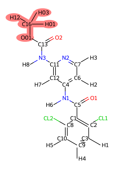
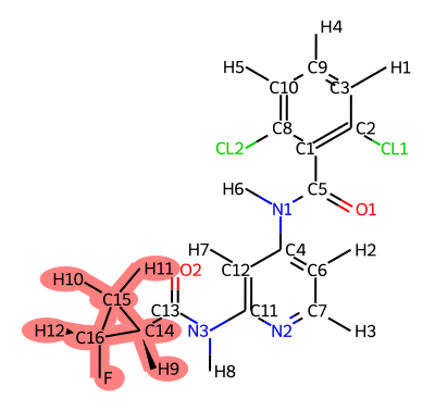
The first step you will want to do is examine the atom mappings for each transformation. While you can do this by hand, we will use the results from the imgdir/ folder created in the results_tyk2/ directory.
cd results_tyk2/imgdir
xdg-open index.html
This will open an HTML file in your web-browser which contains images of the atom mappings for each transformation.
Warning
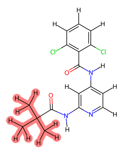
It is important to carefully examine the atom mappings to ensure that they make chemical sense. Soft core regions are highlighted in red.
Rules of Thumb: - There should only be one soft-core region per ligand. - Soft-core regions should contain the entirety of any ring systems being transformed. - Any bonds/angles/dihedrals not involved in soft-core regions will not benefit from ACES enhanced sampling, so if you expect significant conformational changes during the transformation, consider including those regions in the soft-core region.
First open index.html, which will give you an overview of all the transformations.


Modifying Atom Mappings
Now, this is a case where you may want to modify the atom mapping, for instance if you want to enhance sampling of the dihedral leading into the ring system. To do that, you need to know the atom indices of the atoms you want to modify.
You can find these by opening the index_labels.html file in the same imgdir/ folder. This file contains the same images as index.html, but with atom indices labeled.

To do this, make a directory in your working directory for the edited mapping files and copy over the mapping files for each transformation. In the example below we will call this directory coremap.
mkdir coremap
cp tyk2/setup/*map.txt coremap/
This gives you three files - ejm44~ejm55_map.txt, jmc23~ejm44_map.txt, and jmc23~ejm55_map.txt.
Open the mapping file for the transformations you want to modify in a text editor. The mapping file maps atoms in the common_core region between the two ligands. Thus, to increase the soft-core region, we need to remove the atoms we want to include in the soft-core region from the mapping file. We can do this using the labeled images from above.
For example, from ejm_44~ejm_55.map.txt, we can remove the following lines to include the dihedral leading into the ring system in the soft-core region:
O2 =>   O2
H8 =>   H8
N3 =>   N3
C13 =>  C13
Note - while in this case the atom names were the same, this is not always true.
Remove these lines from the remaining mapping files, and save the modified mapping files.
Warning
Be very careful when modifying the mapping files. Ensure that the modified mappings still make chemical sense, and that no bonds are broken in the common core region. Also, ensure that the same atoms are not mapped to different atoms in different transformations involving the same ligand.
Now - to use the new mappings, we need to point the input file to where it can find the new mappings, and then re-run the setup process.
To do this, add the following line to the [ATOM MAPPING] section of your input file:
read_map=coremap
Here, coremap is the name of the directory containing your edited *_map.txt files. If you choose a different directory name, read_map should match that name exactly.
Note
Manual mapping edits are one of the most system-dependent parts of RBFE setup. If a calculation later behaves poorly, this is one of the first places to revisit. Look for mappings that split ring systems awkwardly, leave important torsions outside the soft-core region, or treat the same ligand inconsistently across multiple edges.
Then, re-run the setup process:
rm -rf tyk2
rm -rf results_tyk2
setup_fe
This will re-generate the simulation directories using the modified atom mappings. You can re-examine the mappings in the imgdir/ folder to ensure that the modifications were applied correctly.
Submitting Jobs to the Cluster
To submit the simulations to your cluster, run the following command:
./runalltrials.sh
This is a smart submission script that will try to submit all jobs, and if it fails (e.g. because it hits a job limit), it will keep trying until all jobs are submitted. Trials are submitted as separate jobs to maximize parallelism.
Once all jobs are submitted, you can monitor their progress using your cluster’s job monitoring tools (e.g., squeue, qstat, etc.).
Analyzing Results
Once all simulations are complete, you can analyze the results by changing the stage parameter in your input file from setup to analysis, and re-running setup_fe:
# Edit input file to change stage from setup to analysis
setup_fe
This will perform the analysis of the TI simulations and generate output files in the results_tyk2/ directory.
You can view the analysis results by opening the Graph.html file in the results_tyk2/analysis directory.
xdg-open results_tyk2/analysis/Graph.html # or open on MacOS
We have hosted the file here for your convenience: Graph.html
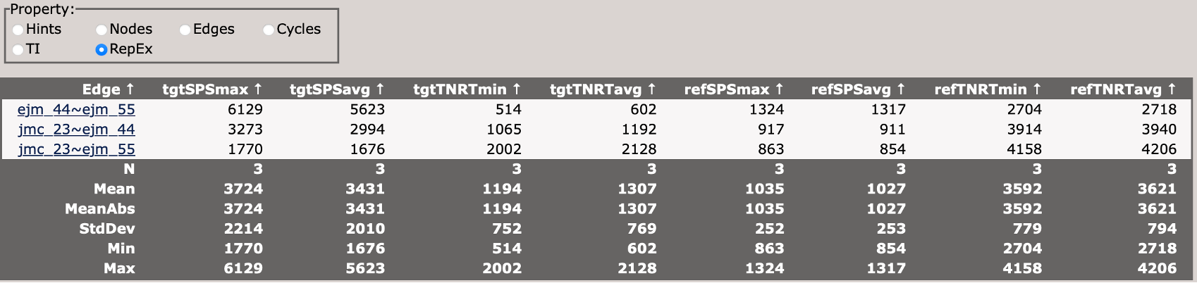
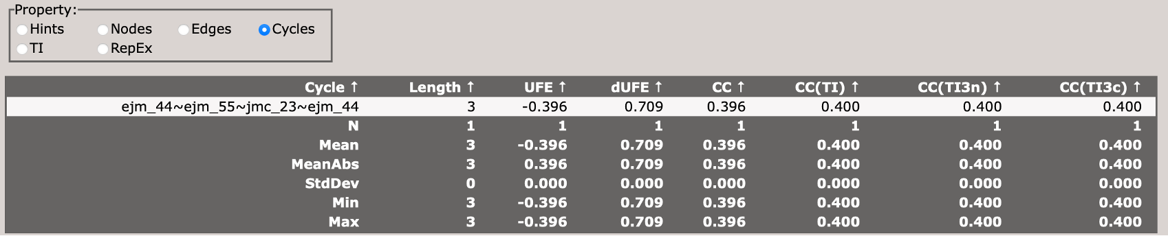
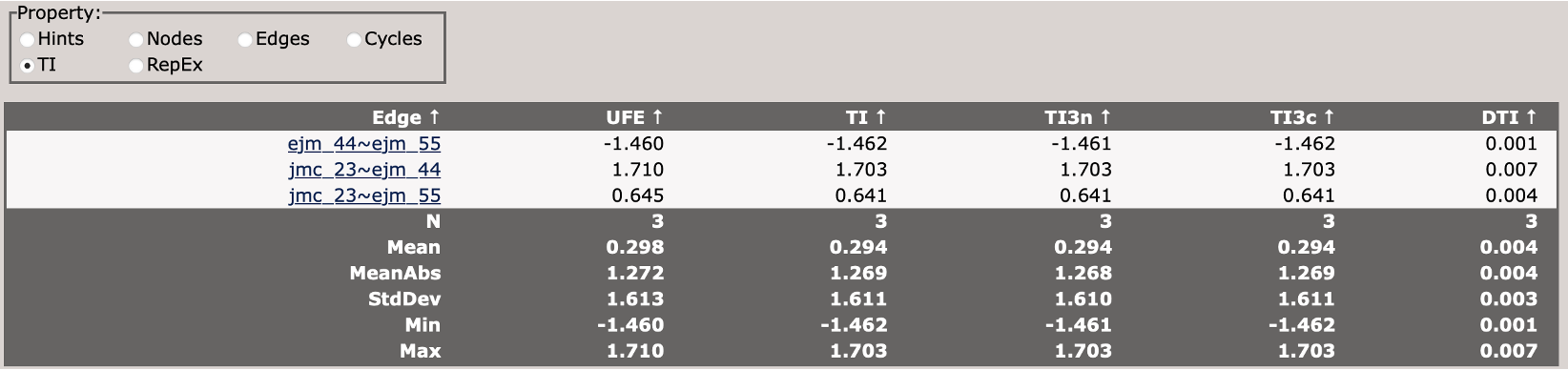
When you first load the HTML file, you will see at the top of the file a map of the RBFE network (in this case three ligands) with a variety of controls.
You can use these controls to customize the display of the results, including the coloring of nodes, and the coloring and thickness of edges based on various metrics.
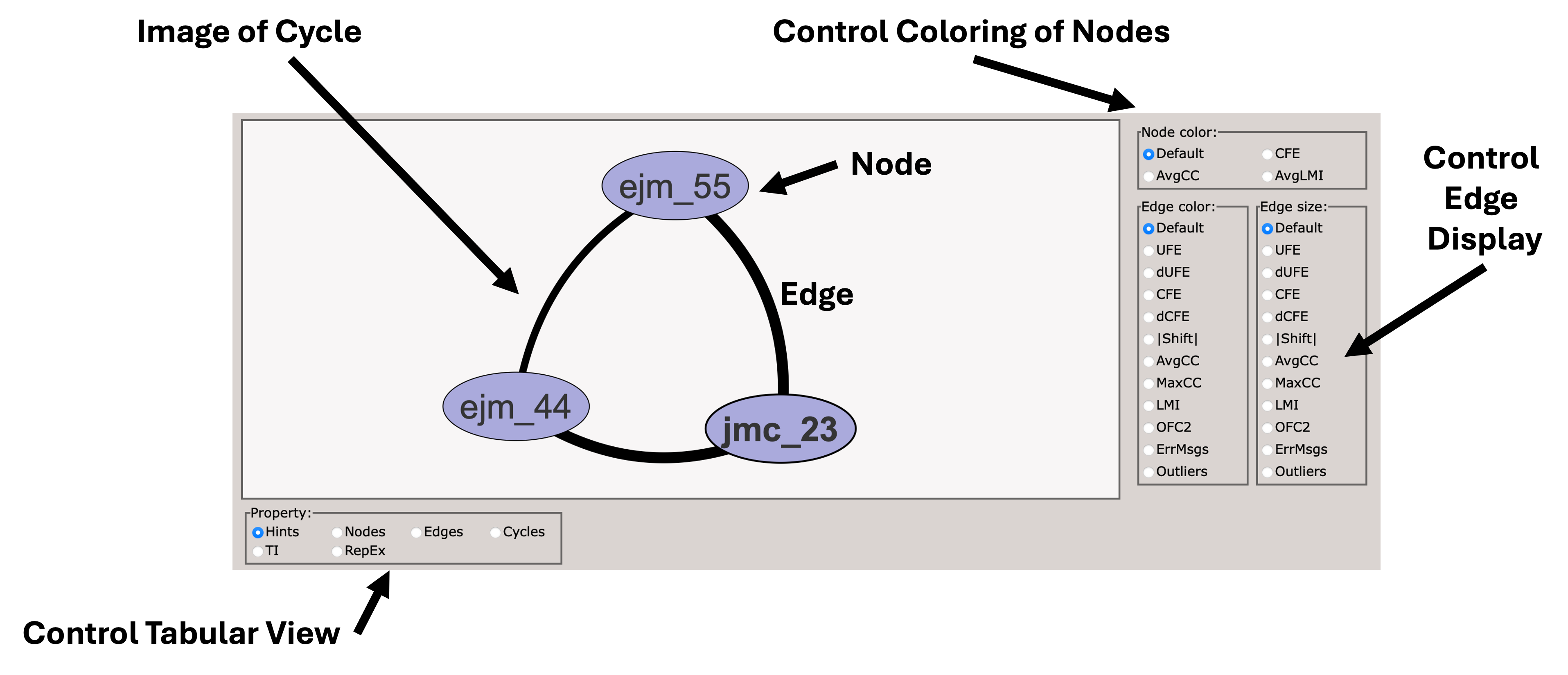
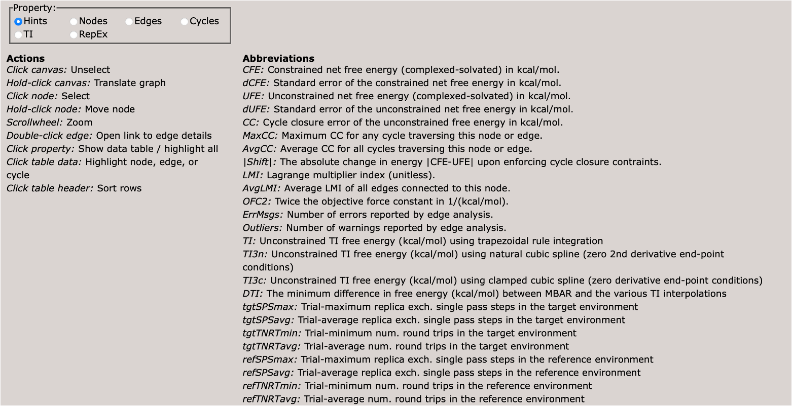
Scrolling down, you will see a control panel that allows you to display a variety of views. The default is a help pane which describes various important abbreviations.
This section describes various important abbreviations used in the graph display.
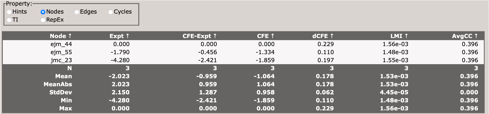
This section describes the free energy of individual nodes (ligands) in the network (relative to an arbitrary reference ligand).
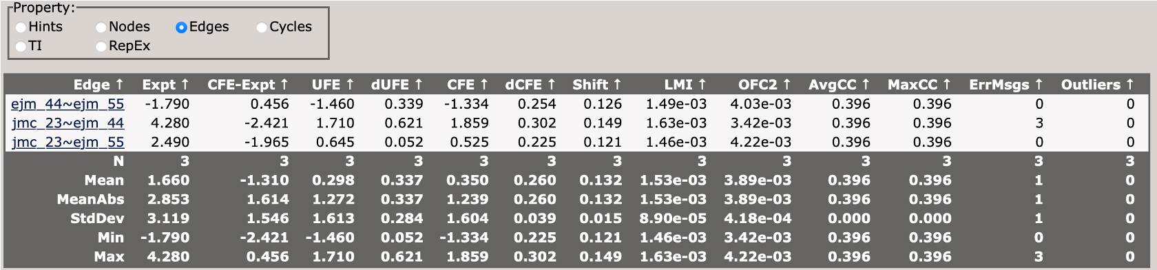
This section describes the free energy differences between pairs of ligands (edges) in the network.
This section describes the cycle closure errors for cycles in the network.
This compares different TI analysis approaches and how well they agree with BAR.
This section describes the replica exchange statistics for each edge in the network.