Linear Dihedral Scans with FFPOPT
Learning objectives
Use FFPOPT to Run Dihedral Scans for a Simple Molecule using the a Linear Scan Method
Activities
        flowchart LR

    InputFile["Input Structure"]
    FFPOPT["ffpopt-DihedScan"]
    Convert["ffpopt-xyz2mol2"]
    Trajectory["Dihedral XYZ Trajectory"]
    EnergyProfile["Dihedral Energy Profile"]

    InputFile --> |parm7 + rst7| FFPOPT
    InputFile --> |mol2| FFPOPT
    InputFile --> |xyz| Convert
    Convert --> FFPOPT

    FFPOPT --> Trajectory
    FFPOPT --> EnergyProfile
In this activity, we will be using a small molecular fragment that contains a deprotonated amide. These fragments can show up in certain ligands, and are presently a challenge for standard force field generation within amber. We will walk through how to use FFPOPT to scan dihedral angles with both MD force-fields and machine learning potentials, and then we will walk through the process of fitting new dihedral parameters.
The files you will need are located here:
Linear Dihedral Scans
In this activity, we will explain how to run linear dihedral scans using FFPOPT. Linear scans are the most straightforward type of dihedral scan, where each dihedral angle is scanned independently one after another. This is done by fixing the dihedral angle at a series of values, and then optimizing the rest of the molecular geometry at each value. The resulting energies can then be used to fit new dihedral parameters.
In the FFPOPT package, these normal types of dihedral scans are called using the ffpopt-DihedScan.py script. This script takes a number of command line arguments, which are described in the help message. You can see the help message by running the following command:
python3 ffpopt-DihedScan.py -h
This will give you a summary of all the available options for running a dihedral scan (note - there are many!)
The main arguments you will need to specify are:
–parm: The path to the AMBER parameter file (parm7) for the molecule you are scanning.
–crd: The path to the AMBER restart file (rst7) for the molecule
–dihed: The dihedral angle(s) to scan, specified as a list of four atom indices (this matches VMD indexing, starting at 0)
–model: The model to use for energy calculations (i.e. sander)
–ase-opt: This is a boolean flag that uses the Atomic Simulation Optimizer rather than the GEOMETRIC optimizer for geometry optimizations (faster, but less robust)
–oscan: The output xyz file for the scan results.
An example command to run a linear dihedral scan using FFPOPT is shown below:
ffpopt-DihedScan.py --parm mmm_NN.parm7 --crd mmm_NN.rst7 --dihed "5,4,3,1" --model sander --ase-opt --oscan linear_scan_5-4-3-1_30deg.xyz --delta 30
Now, here is a breakdown of what each argument does in this example:
–parm mmm_NN.parm7: Specifies the AMBER parameter file for the molecule being scanned.
–crd mmm_NN.rst7: Specifies the AMBER restart file for the molecule.
–dihed “5,4,3,1”: Specifies the dihedral angle to scan, defined by the four atom indices 5, 4, 3, and 1.
–model sander: Specifies that the sander module of AMBER will be used for energy calculations.
–ase-opt: Indicates that the Atomic Simulation Environment (ASE) optimizer will be used for geometry optimizations.
–oscan linear_scan_5-4-3-1_30deg.xyz: Specifies the output file where the scan results will be saved in XYZ format.
–delta 30: Specifies the increment in degrees for each step of the dihedral scan (in this case, 30 degrees).
This command will perform a linear dihedral scan in increments of 30 degrees (since we set delta to 30) for the dihedral defined by atoms 5, 4, 3, and 1. The results of the scan will be saved in the specified output file. A second output file, linear_scan_5-4-3-1_30deg.dat, will also be created, which contains the energies and dihedral angles sampled during the scan.
Note
FFPOPT linear scans actually do two iterations of the scan, one in the positive direction and one in the negative direction. This is done to ensure that the scan captures any potential hysteresis effects, where the energy profile may differ depending on the direction of the scan. The results from both scans are combined into a single output file by taking the minimum energy at each dihedral angle sampled.
Warning
Depending on the system being scanned, linear scans can sometimes miss low-energy conformations due to the sequential nature of the scan. If the molecule has multiple rotatable bonds, it is possible for the geometry optimizer to get stuck in a local minimum, leading to an incomplete exploration of conformational space. In such cases, more advanced scanning methods like WaveFront scans may be more effective.
We can visualize the results fo the scan using VMD, by loading the output xyz file.
vmd linear_scan_5-4-3-1_30deg.xyz
If you play the movie, you should see something that looks very similar to what we see below:
Note
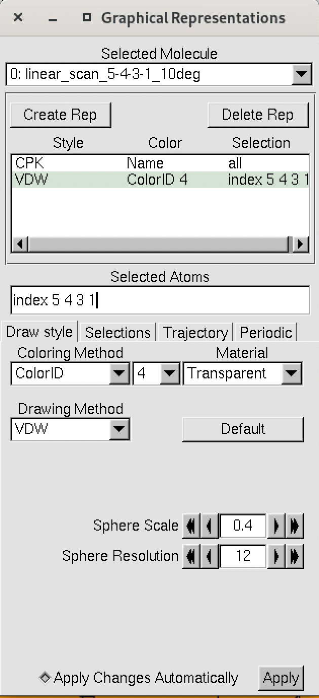
The numbering of the dihedral angles matches the VMD indexing, so the four atoms are selected in VMD as 5, 4, 3, and 1. You can see the selection in VMD below:
Now, we can finally plot the results of the scan using xmgrace or another plotting program, by plotting the data from the dat file.
For instance, using xmgrace, we can run the following command:
xmgrace linear_scan_5-4-3-1_30deg.dat
This will give us a plot of the energy vs dihedral angle, which should look something like this:
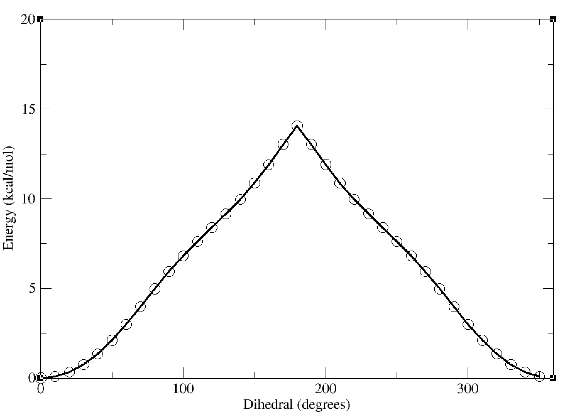
In this case, the dihedral angle is at a minimum at 0 degrees, which corresponds to the planar conformation of the amide. The energy increases as the dihedral angle deviates from this value, reaching a maximum at 180 degrees.