Developing Custom Dihedral Parameters with FFPOPT
Learning objectives
Set up and generate a dihedral-fitting workflow script with ffpopt-DihedTwistWorkflow.py.
Describe the iterative FFPOPT fitting cycle that compares low-level and reference (QDPi2) torsional scans.
Produce updated dihedral parameters and assess improvement of fitted force-field profiles against the reference data.
Activities
        flowchart LR

        InputFile["Input Structure"]
        FFPOPT["ffpopt-DihedTwistWorkflow"]
        Convert["ffpopt-xyz2mol2"]
        HighLevelScan["Wavefront at High-Level"]
        LowLevelScan["Wavefront at Low-Level"]
        ParameterFitting["Fit Parameters"]
        FixParameters["Fixed Parameters Python File"]
        Rescan["Rescan with New Parameters"]
        FinalScan["Final Parameters"]


        InputFile --> |parm7 + rst7| FFPOPT
        InputFile --> |mol2| FFPOPT
        InputFile --> |xyz| Convert
        Convert --> FFPOPT

        FFPOPT --> HighLevelScan
        FFPOPT --> LowLevelScan
        HighLevelScan --> ParameterFitting
        LowLevelScan --> ParameterFitting
        ParameterFitting --> Rescan
        Rescan --> FinalScan
In this activity, we will be using a small molecular fragment that contains a deprotonated amide. These fragments can show up in certain ligands, and are presently a challenge for standard force field generation within amber. We will walk through how to use FFPOPT to scan dihedral angles with both MD force-fields and machine learning potentials, and then we will walk through the process of fitting new dihedral parameters.
The files you will need are located here:
Dihedral Fitting
Often, when parameterizing a new molecule for a molecular dynamics simulation, the default force field parameters will not accurately capture the torsional energy landscape of certain dihedral angles. In these cases, it is necessary to fit new dihedral parameters to better reproduce high-level quantum mechanical calculations or machine learning potential energy surfaces.
In this activity, we will use FFPOPT to fit new dihedral parameters for the deprotonated amide fragment for the GAFF2 force-field, using the QDPI2 machine learning potential as our reference “high-level” method.
Roughly, FFPOPT approaches dihedral fitting in the following way:
Perform a conformational scan of the dihedral(s) of interest using both the existing force field and the reference method (here, QDPI2).
Compare the energy profiles from the force field and the reference method.
Generate primative dihedrals that can be used to fit the difference between the two energy profiles.
Re-calculate the energy profile using the modified force field with the new dihedral parameters.
Iterate the fitting process until the force field energy profile closely matches the reference method.
To get started with this, we will use the Dihedral Twist Workflow, which automates much of this process.
ffpopt-DihedTwistWorkflow.py --parm mmm_NN.parm7 --rst mmm_NN.rst7 --bond "4,3" --delta 10 --nprim 3 --nproc 10 --wf_starting_nodes 4 --geometric-converge 'set GAU' --model qdpi2 > scan.sh
This command will generate a script called scan.sh that contains all the necessary steps to perform the dihedral fitting workflow. You can then run this script to carry out the fitting process. If you explore the scan.sh file, you will see that it contains commands to perform the scans, generate the primative dihedrals, and fit the new parameters.
Opening up the scan.sh file, you will see commands calling the wavefront workflow to perform scans at both they low and high levels of theory, as well as commands to generate new dihedral parameters and run scans on those iteratively until new parameters are reached.
Note
The script, ffpopt-DihedTwistWorkflow.py, has many options that can be adjusted to fit your specific needs, and accepts any arguments that the WaveFront method accepts. You can explore these options by running ffpopt-DihedTwistWorkflow.py –help.
Taking a look at scan.sh, you will see that it contains commands calling the wavefront workflow to perform scans at both they low and high levels of theory, as well as commands to generate new dihedral parameters and run scans on those iteratively until new parameters are reached.
Take a look at the file below that is generated. You’ll see that it contains calls to the wavefront method to perform scans at both the low and high levels of theory, as well as calls to generate new dihedral parameters and run scans on those iteratively until new parameters are reached.
#!/bin/bash
set -e
set -u

# High level scan with QDPi2
if [ ! -e qdpi2_5-4-3-1.xyz ]; then
    echo Creating qdpi2_5-4-3-1.xyz
    ffpopt-DihedWavefront.py -p mmm_NN.parm7 -c mmm_NN.rst7 --model qdpi2 --dihed="5,4,3,1" \
        --oscan qdpi2_5-4-3-1.xyz --delta 10 --nproc 1 --wf_starting_nodes 4 --wf_max_levels -1 --wf_num_conformers 0 --geometric-converge 'set GAU'

fi

# Low level scan with sander
if [ ! -e orig_5-4-3-1.xyz ]; then
    echo Creating orig_5-4-3-1.xyz
    ffpopt-DihedWavefront.py -p mmm_NN.parm7 -c mmm_NN.rst7 --model=sander --dihed="5,4,3,1" \
        --oscan orig_5-4-3-1.xyz --delta 10 --nproc 1 --wf_starting_nodes 4 --wf_max_levels -1 --wf_num_conformers 0 --geometric-converge 'set GAU'

fi

# Iteration 1 Fitting
if [ ! -e it01.py ]; then
    echo Creating it01.py
    ffpopt-GenDihedFit.py --nlmaxiter=300  --ase-opt it01.json
fi

# Make new parm7 with it01.py
if [ ! -e it01.parm7 ]; then
    echo Creating it01.parm7
    python3 it01.py mmm_NN.parm7 it01.parm7
fi


# Calculate updated low level scan with it01.parm7
if [ ! -e it01_5-4-3-1.xyz ]; then
    echo Creating it01_5-4-3-1.xyz
    ffpopt-DihedWavefront.py -p it01.parm7 -c mmm_NN.rst7 --model sander --dihed="5,4,3,1" \
        --oscan it01_5-4-3-1.xyz --delta 10 --nproc 1 --wf_starting_nodes 4 --wf_max_levels -1 --wf_num_conformers 0 --geometric-converge 'set GAU'

fi

# Iteration 2 Fitting
if [ ! -e it02.py ]; then
    echo Creating it02.py
    ffpopt-GenDihedFit.py --nlmaxiter=300  --ase-opt it02.json
fi

# Make new parm7 with it02.py
if [ ! -e it02.parm7 ]; then
    echo Creating it02.parm7
    python3 it02.py mmm_NN.parm7 it02.parm7
fi

# Calculate updated low level scan with it02.parm7
if [ ! -e it02_5-4-3-1.xyz ]; then
    echo Creating it02_5-4-3-1.xyz
    ffpopt-DihedWavefront.py -p it02.parm7 -c mmm_NN.rst7 --model sander --dihed="5,4,3,1" \
        --oscan it02_5-4-3-1.xyz --delta 10 --nproc 1 --wf_starting_nodes 4 --wf_max_levels -1 --wf_num_conformers 0 --geometric-converge 'set GAU'

fi
We can then run this script to carry out the fitting process:
bash scan.sh
This will most likely take a while, depending on your computational resources. Once it is complete, you will have new dihedral parameters that better reproduce the QDPI2 energy profile for the dihedral of interest.
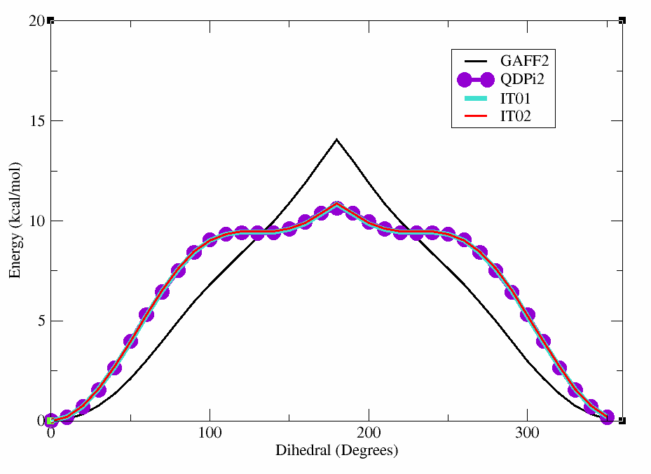
We can plot these results to see how well the new parameters reproduce the reference energy profile.
xmgrace orig_5-4-3-1.xyz qdpi2_5-4-3-1.xyz it01_5-4-3-1.xyz it02_5-4-3-1.xyz
You can see the plot below which shows the original GAFF2 parameters in black, the QDPI2 reference in purple,