Ligand Parameterization Basics
Learning objectives
Perform the basic steps of ligand parameterization by hand using Antechamber, ParmChk2, and tleap.
Look through the files generated by these programs to understand what information is stored where.
Perform ligand parameterization using RESP charge fitting with Antechamber and Gaussian.
Relevant literature
Outline
In this activity we will be covering the basic use of ligand parameterization with LigandParam, a tool developed by the York group to make ligand parameterization easy to do in a way that matches our best practices.
This activity will cover both the old way of doing simple parameterizations by hand, and then show how to do the same thing with LigandParam.
Activities
        flowchart LR
    Start[Start: ligand.pdb]

    subgraph ByHand [Simple AM1-BCC]
        direction LR
        A1[antechamber -c bcc<br/>-> ligand.mol2]
        A2[parmchk2 -f mol2<br/>-> ligand.frcmod]
        A3[tleap -f leap.in<br/>-> ligand.lib]
        A4[python mol2_to_pdb_bfactor.py<br/>-> ligand_charges.pdb]
        A5[VMD visualize_charges.tcl]
    end

    subgraph RESP [RESP charge fitting]
    direction LR
    R1[antechamber -fo gcrt -gv<br/>-> ligand.gjf]
    R2[Gaussian: g16 < ligand.gjf > ligand_run.log]
    R3[antechamber -fi gout -c resp<br/>-> ligand_resp.mol2]
    R4[parmchk2 -i ligand_resp.mol2<br/>-> ligand_resp.frcmod]
    R5[tleap -f leap_resp.in <br/>-> ligand_resp.lib]
    R6[python mol2_to_pdb_bfactor.py<br/>-> resp_charges.pdb]
    end

    Start --> ByHand
    Start --> RESP

    ByHand --> A1 --> A2 --> A3 --> A4 --> A5
    RESP --> R1 --> R2 --> R3 --> R4 --> R5 --> R6

    %% Comparison arrow
    A4 -. Compare .-> R6
    CompareNote[(Compare charges / diff pdb<br/>python pdb_bfactor_diff.py<br/>vmd -e visualize_charges.tcl -args diff.pdb)]
    A4 --> CompareNote
    R6 --> CompareNote

    %% files summary node
    Files[[Files produced:
    - ligand.mol2, ligand.frcmod, ligand.lib
    - ligand.gjf, ligand_run.log, ligand_resp.mol2, ligand_resp.frcmod, ligand_resp.lib
    - ligand_charges.pdb, resp_charges.pdb, diff.pdb
    ]]
    CompareNote --> Files
Parameterizing with AM1-BCC Charges
At the very simplest, a ligand parameterization can be done just with Antechamber, ParmChk2, tleap, as follows.
Start by creating a subdirectory called by_hand, and copy the ligand pdb into that subdirectory from your current working directory.
Note
This activity assumes you have a file called ligand.pdb in your current working directory, this can be any small molecule you want to parameterize. In this activity, we will be working with a minimal ligand that has a net -1 charge.
ATOM      1 N1   LIG A   1       4.400  -0.997   0.000  0.00  0.00           N
ATOM      2 C2   LIG A   1       3.064  -1.169   0.000  0.00  0.00           C
ATOM      3 C3   LIG A   1       2.164  -0.103  -0.000  0.00  0.00           C
ATOM      4 C4   LIG A   1       2.724   1.178  -0.000  0.00  0.00           C
ATOM      5 N5   LIG A   1       4.054   1.386  -0.000  0.00  0.00           N
ATOM      6 C6   LIG A   1       4.815   0.279   0.000  0.00  0.00           C
ATOM      7 C7   LIG A   1       0.679  -0.362  -0.000  0.00  0.00           C
ATOM      8 O7   LIG A   1       0.294  -1.565  -0.001  0.00  0.00           O
ATOM      9 N8   LIG A   1      -0.049   0.760  -0.000  0.00  0.00           N
ATOM     10 C9   LIG A   1      -1.396   0.628  -0.000  0.00  0.00           C
ATOM     11 S10  LIG A   1      -2.272  -0.950  -0.000  0.00  0.00           S
ATOM     12 C11  LIG A   1      -3.705   0.008   0.000  0.00  0.00           C
ATOM     13 N12  LIG A   1      -3.551   1.310   0.000  0.00  0.00           N
ATOM     14 N13  LIG A   1      -2.221   1.672  -0.000  0.00  0.00           N
ATOM     15 O14  LIG A   1      -4.950  -0.558   0.001  0.00  0.00           O
ATOM     16 H2   LIG A   1       2.685  -2.188   0.000  0.00  0.00           H
ATOM     17 H6   LIG A   1       5.893   0.435   0.000  0.00  0.00           H
ATOM     18 H4   LIG A   1       2.075   2.050  -0.000  0.00  0.00           H
ATOM     19 H141 LIG A   1      -5.545   0.220   0.001  0.00  0.00           H
END
mkdir by_hand
cp ligand.pdb by_hand/
cd by_hand
Assume you are starting with ligand.pdb, first you would call antechamber to create a mol2 file with bcc charges.
# Call Antechamber to apply bcc charges to ligand.pdb
# -i : Input file (ligand.pdb)
# -o : Output file (ligand.mol2)
# -fi: Input file format (pdb)
# -fo: Output file format (mol2)
# -c : Charge method (bcc)
# -rn: Residue name (LIG)
# -at: Atom type (gaff2)
# -nc: Net charge (the default ligand for this activity has a net -1 charge)
antechamber -i ligand.pdb -o ligand.mol2 -fi pdb -fo mol2 -c bcc -rn LIG -at gaff2 -nc -1
This command creates a mol2 file with BCC-assigned partial charges next to each atom. If this runs correctly you’ll see something like this:
antechamber -i ligand.pdb -o ligand.mol2 -fi pdb -fo mol2 -c bcc -rn LIG -at gaff2 -nc -1
Info: acdoctor mode is on: check and diagnose problems in the input file.
Info: The atom type is set to gaff2; the options available to the -at flag are
      gaff, gaff2, amber, bcc, abcg2, and sybyl.

-- Check Format for pdb File --
   Status: pass
Info: Bond types are assigned for valence state (1) with penalty (1).

Running: /home/piskulic/Project/SoftwareDevelopment/install_lbsr_dev/bin/sqm -O -i sqm.in -o sqm.out
At the end, you should now have a mol2 for the ligand. The final mol2 should look similar to what you can find below.
@<TRIPOS>MOLECULE
LIG
   19    20     1     0     0
SMALL
bcc


@<TRIPOS>ATOM
      1 N1           4.4000    -0.9970     0.0000 nb         1 LIG      -0.723000
      2 C2           3.0640    -1.1690     0.0000 ca         1 LIG       0.447700
      3 C3           2.1640    -0.1030    -0.0000 ca         1 LIG      -0.292200
      4 C4           2.7240     1.1780    -0.0000 ca         1 LIG       0.447700
      5 N5           4.0540     1.3860    -0.0000 nb         1 LIG      -0.723000
      6 C6           4.8150     0.2790     0.0000 ca         1 LIG       0.605900
      7 C7           0.6790    -0.3620    -0.0000 ce         1 LIG       0.538900
      8 O7           0.2940    -1.5650    -0.0010 o          1 LIG      -0.741300
      9 N8          -0.0490     0.7600    -0.0000 nf         1 LIG      -0.562000
     10 C9          -1.3960     0.6280    -0.0000 cd         1 LIG       0.700400
     11 S10         -2.2720    -0.9500    -0.0000 ss         1 LIG      -0.243800
     12 C11         -3.7050     0.0080     0.0000 cd         1 LIG       0.441700
     13 N12         -3.5510     1.3100     0.0000 nc         1 LIG      -0.413000
     14 N13         -2.2210     1.6720    -0.0000 nc         1 LIG      -0.416000
     15 O14         -4.9500    -0.5580     0.0010 oh         1 LIG      -0.611300
     16 H2           2.6850    -2.1880     0.0000 h4         1 LIG       0.052600
     17 H6           5.8930     0.4350     0.0000 h5         1 LIG       0.031100
     18 H4           2.0750     2.0500    -0.0000 h4         1 LIG       0.052600
     19 H141        -5.5450     0.2200     0.0010 ho         1 LIG       0.408000
@<TRIPOS>BOND
     1     1     2 ar
     2     1     6 ar
     3     2     3 ar
     4     2    16 1
     5     3     4 ar
     6     3     7 1
     7     4     5 ar
     8     4    18 1
     9     5     6 ar
    10     6    17 1
    11     7     8 1
    12     7     9 2
    13     9    10 1
    14    10    11 1
    15    10    14 2
    16    11    12 1
    17    12    13 2
    18    12    15 1
    19    13    14 1
    20    15    19 1
@<TRIPOS>SUBSTRUCTURE
     1 LIG         1 TEMP              0 ****  ****    0 ROOT
Hint
A quick refresher on the mol2 format.
The mol2 format is a widely used file format for representing molecular structures. It contains information about the atoms, bonds, and other molecular features. The key sections of a mol2 file include:
@<TRIPOS>MOLECULE: This section provides general information about the molecule, including its name, number of atoms, and other properties.
@<TRIPOS>ATOM: This section lists all the atoms in the molecule, along with their coordinates, atom types, and partial charges.
@<TRIPOS>BOND: This section defines the bonds between atoms, including bond types and connectivity.
@<TRIPOS>SUBSTRUCTURE: This section describes any substructures within the molecule, such as functional groups or rings.
Now, its important to note that antechamber writes a mol2 file with amber atom types instead of elements.
This means that when you are looking at the mol2 file, you should pay attention to the atom types and ensure they match the expected amber types.
Now, we need to create a frcmod file from the mol2 file. The frcmod file contains additional force field parameters that are not present in the mol2 file or the GAFF2 forcefield.
# Call ParmChk2 to create a frcmod file from the mol2 file
# -i : Input file (ligand.mol2)
# -o : Output file (ligand.frcmod)
# -f : Input file format (mol2)
# -s : ff parm set (2, which is equivalent to gaff2)

parmchk2 -i ligand.mol2 -o ligand.frcmod -f mol2 -s 2
If everything runs as expected, you should get no output to your screen and you should see a file ligand.frcmod appear in your filesystem.
The contents of that file can be seen below.
Remark line goes here
MASS

BOND

ANGLE
ca-ce-o    79.900     121.180   same as ce-ce-o , penalty score=  2.2
cd-nf-ce   84.130     112.590   same as cd-ne-ce, penalty score=  1.0
nf-ce-o    89.540     125.450   same as ne-cf-o , penalty score= 11.9
oh-cd-ss   78.580     119.440   same as os-cd-ss, penalty score=  2.0

DIHE
ca-ca-ce-o    4    2.800       180.000           2.000      same as X -c2-ca-X , penalty score=237.0
ca-ca-ce-nf   4    4.000       180.000          -2.000      same as ca-ce-ce-n2
ca-ca-ce-nf   1    0.750       180.000          -3.000      same as ca-ce-ce-n2
ca-ca-ce-nf   1    0.820       180.000           1.000      same as ca-ce-ce-n2, penalty score=638.0
ca-ce-nf-cd   1    0.400         0.000           3.000      same as c2-ce-ne-c2, penalty score=312.0
ss-cd-nf-ce   2    1.600       180.000           2.000      same as X -cf-nf-X , penalty score=136.0
nc-cd-nf-ce   2    1.600       180.000           2.000      same as X -cf-nf-X , penalty score=136.0
o -ce-nf-cd   2    1.600       180.000           2.000      same as X -ce-ne-X , penalty score=138.0
nf-cd-ss-cd   2    3.200       180.000           2.000      same as n2-c2-ss-ca, penalty score=406.0
nc-cd-ss-cd   2    3.200       180.000           2.000      same as n2-c2-ss-ca, penalty score=406.0
oh-cd-ss-cd   2    2.200       180.000           2.000      same as X -c2-ss-X , penalty score=232.0
ss-cd-oh-ho   2    2.100       180.000           2.000      same as X -c2-oh-X , penalty score=232.0
nc-cd-oh-ho   2    2.100       180.000           2.000      same as X -c2-oh-X , penalty score=232.0

IMPROPER
ca-h4-ca-nb        10.5          180.0         2.0          Same as X -X -cc-X , penalty score= 41.9 (use general term))
ca-ca-ca-ce         1.1          180.0         2.0          Same as c2-ca-ca-ca, penalty score= 61.9)
h5-nb-ca-nb        10.5          180.0         2.0          Same as X -X -cc-X , penalty score= 41.9 (use general term))
ca-nf-ce-o         10.5          180.0         2.0          Same as X -X -cc-X , penalty score= 37.0 (use general term))
nc-nf-cd-ss        10.5          180.0         2.0          Using general improper torsional angle  X- X-cd- X, penalty score=  9.0)
nc-oh-cd-ss        10.5          180.0         2.0          Using general improper torsional angle  X- X-cd- X, penalty score=  9.0)

NONBON
You’ll see that there are a number of different sections. The MASS and BOND sections are empty, because those are all described by the GAFF2 forcefield that we are using.
The ANGLE, DIHE, and IMPROPER sections all contain entries that were not found in the standard GAFF2 forcefield, so parmchk2 has generated parameters for them based on similar parameters found in the forcefield. The quality of those dihedral parameters is assessed by the penalty score, with lower scores indicating better confidence in the parameters. For terms that have high penalty scores, you might want to consider using electronic sturcture or machine-learning based approaches to improve their parameters.
Note
These are not the only parameters that describe bonded/angular/dihedral interactions - the standard forcefields have files shipped with amber that define their parameters (located in amber/data/leap/gaff2.dat for gaff2).
Now that we have base intramolecular force-field parameters, the last thing we need is a lib file. These files store those partial charges that we provided earlier so that if you are building a system from a docked structure you aren’t forced to re-generate a mol2 with the correct coordinates and can use a pdb instead.
Now we need to create the lib file, to do that we will use a program called tleap.
Write a quick file, called tleap.in, that contains the following commands.
source leaprc.gaff2
loadamberparams ligand.frcmod
LIG = loadmol2 ligand.mol2

saveOff LIG ligand.lib
quit
Now, we can run tleap on this file as:
tleap -f leap.in
When you run this, you will see output on your screen that looks something like this.
-I: Adding /home/piskulic/Project/SoftwareDevelopment/install_lbsr_dev/dat/leap/prep to search path.
-I: Adding /home/piskulic/Project/SoftwareDevelopment/install_lbsr_dev/dat/leap/lib to search path.
-I: Adding /home/piskulic/Project/SoftwareDevelopment/install_lbsr_dev/dat/leap/parm to search path.
-I: Adding /home/piskulic/Project/SoftwareDevelopment/install_lbsr_dev/dat/leap/cmd to search path.
-f: Source tleap.in.

Welcome to LEaP!
(no leaprc in search path)
Sourcing: ./tleap.in
----- Source: /home/piskulic/Project/SoftwareDevelopment/install_lbsr_dev/dat/leap/cmd/leaprc.gaff2
----- Source of /home/piskulic/Project/SoftwareDevelopment/install_lbsr_dev/dat/leap/cmd/leaprc.gaff2 done
Log file: ./leap.log
Loading parameters: /home/piskulic/Project/SoftwareDevelopment/install_lbsr_dev/dat/leap/parm/gaff2.dat
Reading title:
AMBER General Force Field for organic molecules (Version 2.2.30, Oct 2025)
Loading parameters: ./ligand.frcmod
Reading force field modification type file (frcmod)
Reading title:
Remark line goes here
Loading Mol2 file: ./ligand.mol2
Reading MOLECULE named LIG
 Creating ligand.lib
Building topology.
Building atom parameters.
        Quit

Exiting LEaP: Errors = 0; Warnings = 0; Notes = 0.
Everytime you parameterize with tleap, you should check the Errors and Warnings section to see whether any issues were reported. This can help you catch potential problems early and ensure that your parameterization is as accurate as possible.
Now - lets visualize the charges using a simple python script and VMD. Note - you may want to work on this on your local machine, due to occaisional challenges with X forwarding.
#!/usr/bin/env python3
"""
mol2_to_pdb_bfactor.py

Usage:
    python mol2_to_pdb_bfactor.py input.mol2 output.pdb [--resname MOL] [--write-types types.txt]

What it does:
 - Parses the @<TRIPOS>ATOM block of a mol2 file.
 - Extracts: atom_id, atom_name, x, y, z, atom_type, partial_charge
 - Writes a simple single-residue PDB where the B-factor column contains the partial_charge.
 - Optionally writes a text file mapping atom_index -> atom_type (AMBER atom type stored in mol2 atom_type).
"""

import sys
import argparse
import re

def parse_mol2_atoms(mol2_path):
    atoms = []
    in_atoms = False
    with open(mol2_path, 'r') as fh:
        for line in fh:
            if line.startswith('@<TRIPOS>ATOM'):
                in_atoms = True
                continue
            if line.startswith('@<TRIPOS>'):
                if in_atoms:
                    break
            if not in_atoms:
                continue
            # Typical ATOM line: id name x y z type charge [subst_id subst_name ...]
            parts = line.strip().split()
            if len(parts) < 6:
                continue
            atom_id = parts[0]
            atom_name = parts[1]
            try:
                x = float(parts[2])
                y = float(parts[3])
                z = float(parts[4])
            except ValueError:
                # skip malformed line
                continue
            atom_type = parts[5]
            # charge usually last token (but sometimes additional tokens exist)
            charge = None
            # find a token that parses as float from the end
            for tok in reversed(parts):
                try:
                    charge = float(tok)
                    break
                except:
                    continue
            if charge is None:
                charge = 0.0
            atoms.append({
                'id': atom_id,
                'name': atom_name,
                'x': x, 'y': y, 'z': z,
                'type': atom_type,
                'charge': charge
            })
    return atoms

def guess_element(atom_name, atom_type):
    # Simple heuristics: element is first char(s) of atom_name or atom_type
    # prefer explicit element-like prefixes: C, N, O, H, S, P, CL, BR, F, I
    el = None
    # from atom name
    m = re.match(r'^([A-Za-z]{1,2})', atom_name)
    if m:
        cand = m.group(1)
        cand = cand.capitalize()
        if cand in ("C","N","O","H","S","P","Cl","Br","F","I"):
            return cand.upper()
        # handle 'CA' -> C? (could be alpha carbon) but prefer single-letter if ambiguous
        if cand[0].upper() in "CNOHSPFIBrcl":
            return cand[0].upper()
    # fallback to atom_type prefix
    if atom_type:
        m2 = re.match(r'^([A-Za-z]{1,2})', atom_type)
        if m2:
            return m2.group(1).upper()
    # default C
    return 'C'

def write_pdb(atoms, out_path, resname='MOL'):
    """
    Write PDB with one residue (resSeq 1), chain A.
    B-factor column will be set to the partial charge.
    Atom name uses the mol2 atom name (padded/truncated to 4).
    """
    with open(out_path, 'w') as out:
        atom_idx = 1
        for a in atoms:
            element = guess_element(a['name'], a['type'])
            # Format PDB ATOM line (fixed-column). Keep it simple.
            atom_name = a['name'][:4].rjust(4)
            altLoc = ''
            resName = resname[:3].rjust(3)
            chainID = 'A'
            resSeq = 1
            x = a['x']
            y = a['y']
            z = a['z']
            occupancy = 1.00
            bfactor = a['charge']  # this is the important part
            # build formatted line: columns as in PDB ATOM format
            # Example format:
            # ATOM  %5d %4s %3s %1s%4d    %8.3f%8.3f%8.3f%6.2f%6.2f          %2s
            line = ("ATOM  {atom_idx:5d} {atom_name:<4s}{resName:>3s} {chainID:1s}"
                    "{resSeq:4d}    {x:8.3f}{y:8.3f}{z:8.3f}{occupancy:6.2f}{bfactor:6.2f}          {element:>2s}\n").format(
                atom_idx=atom_idx,
                atom_name=atom_name,
                resName=resName,
                chainID=chainID,
                resSeq=resSeq,
                x=x, y=y, z=z,
                occupancy=occupancy,
                bfactor=bfactor,
                element=element
            )
            out.write(line)
            atom_idx += 1
        out.write("END\n")

def write_types_file(atoms, types_path):
    with open(types_path, 'w') as fh:
        for i,a in enumerate(atoms, start=1):
            fh.write(f"{i}\t{a['name']}\t{a['type']}\t{a['charge']:.6f}\n")

def main():
    parser = argparse.ArgumentParser(description="Convert mol2 -> pdb with B-factor = partial charge")
    parser.add_argument('mol2', help='input mol2 file')
    parser.add_argument('pdb', help='output pdb file')
    parser.add_argument('--resname', default='MOL', help='Residue name to use in PDB (default MOL)')
    parser.add_argument('--write-types', help='Optional: write atom index -> atom type mapping to this file')
    args = parser.parse_args()

    atoms = parse_mol2_atoms(args.mol2)
    if not atoms:
        print("No atoms found in mol2 file or parsing failed.", file=sys.stderr)
        sys.exit(2)
    write_pdb(atoms, args.pdb, resname=args.resname)
    if args.write_types:
        write_types_file(atoms, args.write_types)
    print(f"Wrote {len(atoms)} atoms to {args.pdb}")
    if args.write_types:
        print(f"Wrote atom type mapping to {args.write_types}")

if __name__ == '__main__':
    main()
This python script can be run on your mol2 file to produce a pdb file with B-factors set to the partial charges of the atoms. To run it, do as follows:
python mol2_to_pdb_bfactor.py ligand.mol2 ligand_charges.pdb
You’ll see an output file, ligand_charges.pdb.
Now you can visualize the charges using VMD or any other molecular visualization tool.
You can either do this by hand, OR, you can use the provided VMD tcl script below.
# visualize_charges.tcl

if {[llength $argv] < 1} {
    puts "Usage: vmd -e visualize_charges.tcl -args molecule.pdb [min] [max]"
    exit
}

set pdbfile [lindex $argv 0]
set user_min ""
set user_max ""

if {[llength $argv] >= 3} {
    set user_min [lindex $argv 1]
    set user_max [lindex $argv 2]
}

# Load molecule
mol new $pdbfile type pdb waitfor all
set molID [molinfo top]

# Delete default rep
mol delrep 0 $molID

# Add new representation
mol representation CPK 1.0
mol selection all
mol material Opaque
mol addrep $molID

# IMPORTANT PART: set coloring method on rep 0
mol modcolor 0 $molID Beta

# Optional: set color scale range
if {$user_min ne "" && $user_max ne ""} {
    mol scaleminmax $molID 0 $user_min $user_max
    puts "Color scale set to $user_min .. $user_max"
}

# Optional: show color scale bar (GUI only)
catch {colorbar show}

display resetview
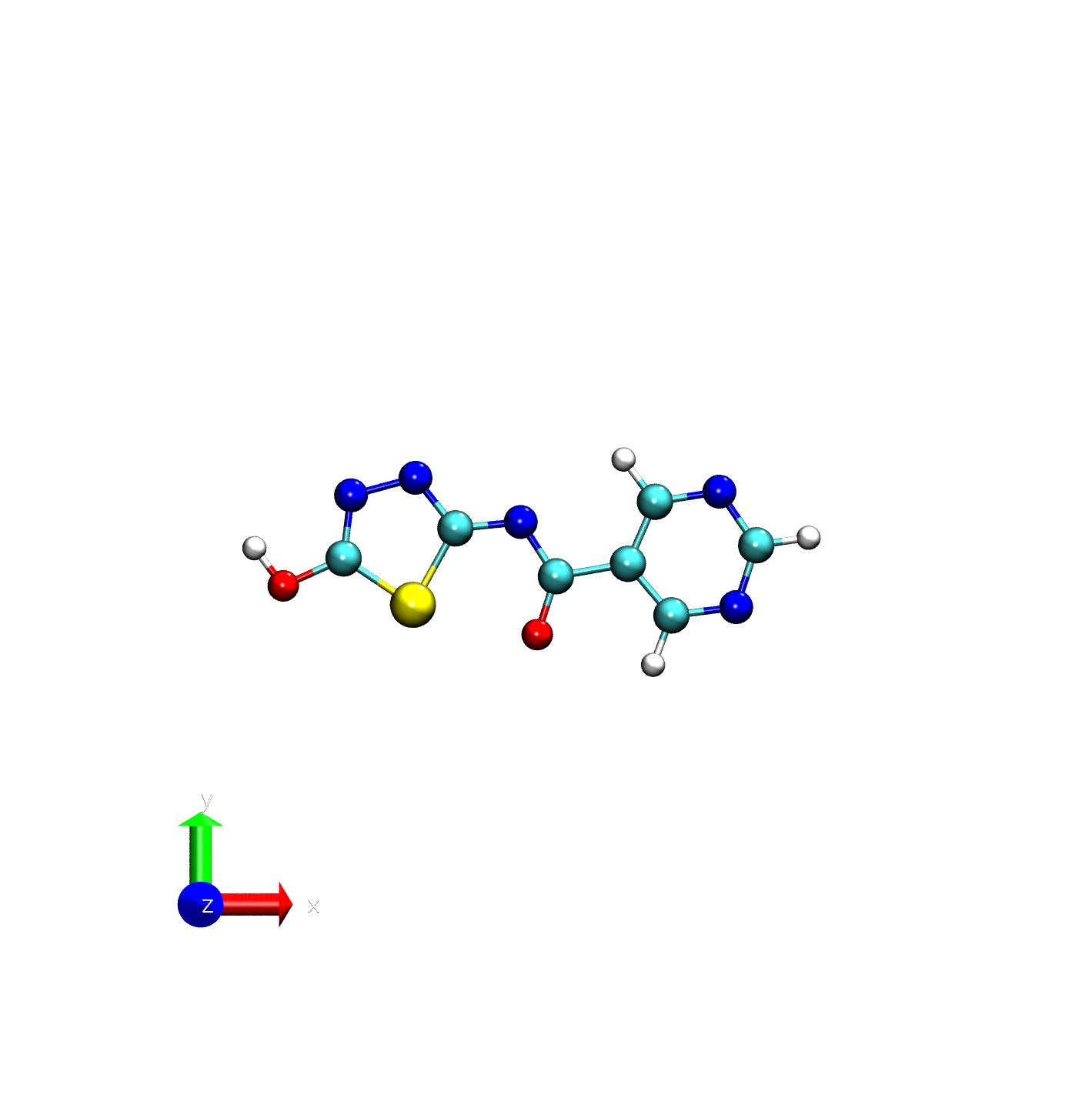
vmd -e visualize_charges.tcl -args ligand_charges.pdb -1.0 1.0
If things worked out - you should see something like this.
Here, we are defining the color range for the visualization, with -1.0 being the minimum and 1.0 being the maximum.
Now this is an easy parameterization, and this already involves running three different programs: antechamber, parmchk2, and tleap. Now imagine you add in the by-hand adjustments described above, and also add in RESP charge fitting. It is pretty clear that this process can get complicated quickly, it is easy to make mistakes, and keeping track of all the different files and parameters can be challenging.
Parameterizing with RESP Charges
Warning
This section requires access to the Gaussian Electronic Structure Program. If you do not have access to Gaussian, you can skip this section and move on to the LigandParam activity.
On {{DISPLAY_NAME}}, Gaussian is available through the following command:
{{GAUSSIAN_LOAD}}
Warning
Gaussian runs take up quite a few resources and should not be run on a login node. Please request an interactive node if you are going to follow along with this activity.
{{INTERACTIVE_REQUEST}}
One of the problems with AM1-BCC charges is that they are not always very accurate, especially for molecules with unusual electronic structures. A better way to get partial charges is to use RESP charge fitting, which fits charges to reproduce the electrostatic potential around the molecule as calculated by a quantum chemistry program. This is a more involved process, but can yield much better results.
Lets go through the steps to do this. We will start from the same pdb file that we used above.
Lets set up a working directory for RESP charge fitting. Again,:term:ligand.pdb <.pdb> should be located in your working directory.
mkdir -p resp_charge_fitting
cd resp_charge_fitting
cp ../ligand.pdb .
First, we need to generate a Gaussian input file to calculate the electrostatic potential. We can do this with antechamber as follows:
# Antechamber to generate Gaussian input file
# -i input file
# -fi input file format
# -o output file
# -fo output file format
# -gv Gaussian adds keyword to generate Gaussian input file
# -ge Gaussian output file
# -nc net charge
# -at atom type
antechamber -i ligand.pdb -fi pdb -o ligand.gjf -fo gcrt -gv 1 -ge ligand.log -nc -1 -at gaff2
The options here are the same as before, with the addition of the gaussian options , which tells antechamber to generate a Gaussian input file for calculating the electrostatic potential.
Note
Details on Gaussian Input File
The generated Gaussian input file (ligand.gjf) looks like this.
--Link1--
%chk=molecule
#HF/6-31G* SCF=tight Test Pop=MK iop(6/33=2) iop(6/42=6) opt
# iop(6/50=1)

remark line goes here

-1   1
    N    4.4000000000       -0.9970000000        0.0000000000
    C    3.0640000000       -1.1690000000        0.0000000000
    C    2.1640000000       -0.1030000000       -0.0000000000
    C    2.7240000000        1.1780000000       -0.0000000000
    N    4.0540000000        1.3860000000       -0.0000000000
    C    4.8150000000        0.2790000000        0.0000000000
    C    0.6790000000       -0.3620000000       -0.0000000000
    O    0.2940000000       -1.5650000000       -0.0010000000
    N   -0.0490000000        0.7600000000       -0.0000000000
    C   -1.3960000000        0.6280000000       -0.0000000000
    S   -2.2720000000       -0.9500000000       -0.0000000000
    C   -3.7050000000        0.0080000000        0.0000000000
    N   -3.5510000000        1.3100000000        0.0000000000
    N   -2.2210000000        1.6720000000       -0.0000000000
    O   -4.9500000000       -0.5580000000        0.0010000000
    H    2.6850000000       -2.1880000000        0.0000000000
    H    5.8930000000        0.4350000000        0.0000000000
    H    2.0750000000        2.0500000000       -0.0000000000
    H   -5.5450000000        0.2200000000        0.0010000000

ligand.log

ligand.log
Lets go through these sections:
- The first section contains the Gaussian route section, which specifies the level of theory and basis set to be used (HF/6-31G*), as well as other options for the calculation.
SCF=tight: Tight convergence criteria for the self-consistent field (SCF) procedure.
Test: This is a keyword that tells Gaussian to perform a test calculation.
Pop=MK: This specifies that the electrostatic potential should be calculated using the Merz-Kollman scheme.
iop(6/33=2): This option specifies that the electrostatic potential should be calculated on a grid of points around the molecule.
iop(6/42=6): This option specifies that the electrostatic potential should be calculated using a grid spacing of 0.2 angstroms.
opt: This tells Gaussian to optimize the geometry of the molecule before calculating the electrostatic potential.
iop(6/50=1): This option specifies that the electrostatic potential should be calculated using a single point calculation.
The second section is a comment line, which can be used to describe the calculation. “remark line goes here”
The third section contains the charge and multiplicity of the molecule. In this case, the molecule has a net charge of -1 and a multiplicity of 1 (singlet state).
The fourth section contains the Cartesian coordinates of the atoms in the molecule.
Now, there are a few modifications you can make if you are interested in doing so.
You can add %mem=10GB to in crease the memory allocated for the Gaussian job.
You can add %nproc=2 to specify that you want to use multiple processors
You can add p after the # to indicate that you want to use the parallel version of Gaussian (right before HF/6-31G*, as #p HF/6-31G* …)
Next, we need to run Gaussian on this input file to generate the electrostatic potential. This can be done with the following command:
g16 < ligand.gjf > ligand_run.log
This will run Gaussian and output the results to ligand.log. Once this is done, we can use antechamber again to extract the electrostatic potential and fit RESP charges.
Warning
This will take some time! On 10 cores, this took 42 minutes on our test system.
Now we will take ligand_run.log and use it to generate the RESP charges.
antechamber -i ligand_run.log -o ligand_resp.mol2 -fi gout -fo mol2 -c resp -rn LIG -at gaff2 -nc -1
Now lets compare the charges generated by RESP to those generated by AM1-BCC. You can do this by looking at the mol2 files generated in each case.
Finally, we can generate the frcmod and lib files as before, using the RESP-charged mol2 file.
parmchk2 -i ligand_resp.mol2 -o ligand_resp.frcmod -f mol2 -s 2
Then create tleap.in again.
# tleap input file
source leaprc.gaff2
loadamberparams ligand_resp.frcmod
LIG = loadmol2 ligand_resp.mol2

saveOff LIG ligand_resp.lib
quit
And run tleap.
tleap -f leap.in
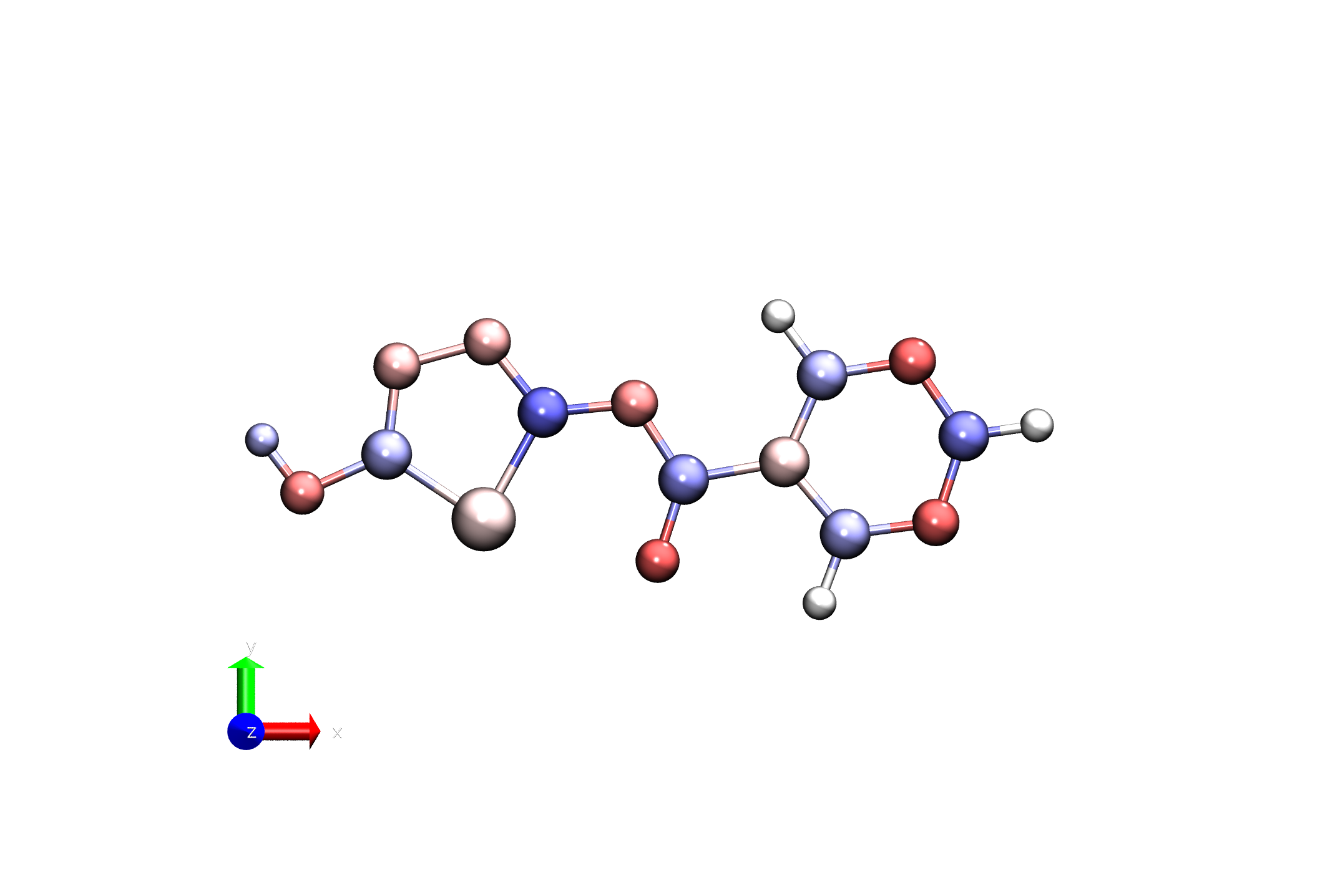
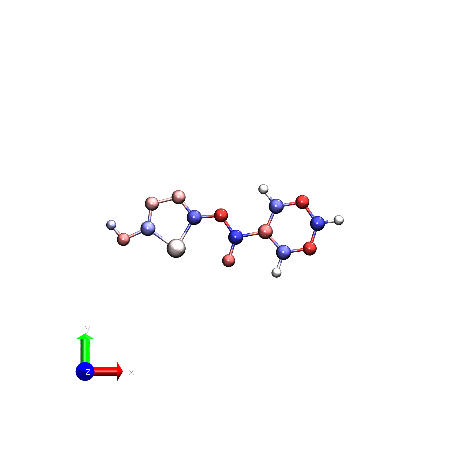
Like before, we can visualize the ligand in VMD using the same procedure as above.
python mol2_to_pdb_bfactor.py ligand_resp.mol2 resp_charges.pdb
vmd -e visualize_charges.tcl -args resp_charges.pdb -1.0 1.0
You can see that the RESP charges have the nitrogens a bit more negatively charged than the AM1-BCC charges.
To make this clearer, we can visualize the difference in charges between the two methods.
To do this, you can use this python code on the two pdb files generated with AM1-BCC and RESP.
Save this file as pdb_bfactor_diff.py.
#!/usr/bin/env python3
"""
pdb_bfactor_diff.py

Compute B-factor differences between two PDBs:
    DeltaB = B_factor(pdb2) - B_factor(pdb1)

Usage:
    python pdb_bfactor_diff.py ref.pdb target.pdb diff.pdb

Assumptions:
 - Same number of atoms
 - Same atom ordering (same serial numbers)
"""

import sys

def read_pdb_atoms(pdb_path):
    atoms = []
    with open(pdb_path, 'r') as fh:
        for line in fh:
            if line.startswith(("ATOM  ", "HETATM")):
                try:
                    serial = int(line[6:11])
                    bfactor = float(line[60:66])
                except ValueError:
                    continue
                atoms.append({
                    "line": line.rstrip("\n"),
                    "serial": serial,
                    "bfactor": bfactor
                })
    return atoms

def write_pdb_diff(atoms1, atoms2, out_path):
    if len(atoms1) != len(atoms2):
        raise RuntimeError("PDB files have different numbers of atoms")

    with open(out_path, 'w') as out:
        for a1, a2 in zip(atoms1, atoms2):
            if a1["serial"] != a2["serial"]:
                raise RuntimeError(
                    f"Atom serial mismatch: {a1['serial']} vs {a2['serial']}"
                )

            delta_b = a2["bfactor"] - a1["bfactor"]

            # Replace B-factor field (columns 61–66)
            line = a1["line"]
            new_line = (
                line[:60] +
                f"{delta_b:6.2f}" +
                line[66:]
            )
            out.write(new_line + "\n")

        out.write("END\n")

def main():
    if len(sys.argv) != 4:
        print("Usage: python pdb_bfactor_diff.py pdb1.pdb pdb2.pdb diff.pdb")
        sys.exit(1)

    pdb1, pdb2, out_pdb = sys.argv[1:]

    atoms1 = read_pdb_atoms(pdb1)
    atoms2 = read_pdb_atoms(pdb2)

    if not atoms1 or not atoms2:
        print("Error: failed to read atoms from one or both PDBs")
        sys.exit(2)

    write_pdb_diff(atoms1, atoms2, out_pdb)
    print(f"Wrote B-factor difference PDB: {out_pdb}")

if __name__ == "__main__":
    main()
You can run this script with the following command.
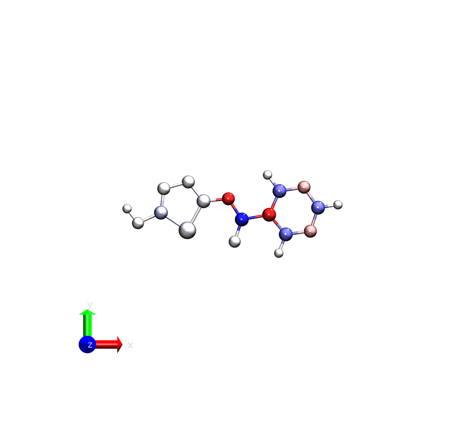
python pdb_bfactor_diff.py ../ligand_charges.pdb resp_charges.pdb diff.pdb
 vmd -e visualize_charges.tcl -args diff.pdb -0.2 0.2
Note that we’ve reduced the range for the color scale since we are now examining the difference
Note
Because RESP calculates charges based on a finite grid around the molecule, the charges that are calculated can be sensitive to the orientation of the molecule. It is often a good idea to run RESP multiple times with different orientations and average the results to get more reliable charges. However, this requires customized programs or scripts to do so and is out of the scope of this activity. See the ligandparam activity for an automated way to do this more complicated procedure.