Analyzing a surface generated with the Surface Accelerated String Method (SASM)
Learning objectives
Analyze the surface from a 2D reaction within MTR1 using the SASM
Relevant literature
Analyzing a set of strings
Now that you understand how the data was generated, you will see how the string has progressed and the resulting free energy surface. The output of the string simulations is located in the outputs directory for the respective initial guesses. You will perform the analysis on the outputs of the string, so these should be copied to your working directory.
For instance, if you are working with the linear initial guess, copy those outputs to your working directory:
[user@cluster] cp -r /expanse/projects/qstore/amber_ws/tutorials/QMMM_DFTB3_MTR1/2D/linear/output ./
[user@cluster] cd output
The outputs contain iterations zero (init) through 20, and each iteration contains a directory called analysis. For the init, it002, it005, it010, and it020 directories, the analysis directory has been moved to analysis-out so that you can generate analysis on your own without writing over files, and if you encounter issues, the intended results are still available for you to look at. For the sake of file size, structure files have been removed, but would have been generated by the simulations. For each of these directories you will run the following series of commands. In each case, replace the –curit flag and change the cd command to the directory you are analyzing. When running Example2d.py, change the title to match the iteration, and use the flag –inset-bright instead of –inset-tleft if you are analyzing the MT initial guess of the path.
Check the equilibration, and create the new dumpave files and metafile:
[user@cluster] ndfes-path-analyzesims.py --curit=0 -d template/img.disang --neqit=4 --temp=298 --maxeq=0.25 --skipg
Go to the analysis directory
[user@cluster] cd init/analysis
Create the chk file:
[user@cluster] ndfes_omp --mbar -w 0.15 --nboot 0 -c metafile.all.chk metafile.all
Optimize the path on the free energy surface:
[user@cluster] ndfes-path_omp --ipath metafile.current --chk metafile.all.chk --neqit=4 --temp 298 --maxit=300 --minsize=10 --akima --npathpts=100 --wavg=4 --wavg-niter=1 --opath path
Create an image of the free energy surface and current estimate of the path:
[user@cluster] python ../../Example2d.py --ipath path.wavg.0.dat --title 'init' --inset-tleft --zerobypath0 --wavg=4 --wavg-niter=1 --minene=-25 --maxene=25 --minsize=10 metafile.all.chk
The ndfes-path-analyzesims.py and ndfes_omp commands are the same as in the SASM run script. For each window, the ndfes-path-analyzesims.py script will print some information about the equilibration of the window. More information can be found by running:
ndfes-CheckEquil.py -h
     Ninp:  The number of input samples
     Nout:  The number of output samples
     Teq:   The percentage of samples excluded as equilibration
     i0:    The 1-based index of the first frame to write (the "start" value
            when using cpptraj)
     s:     The stride through the data (the "offset" value when using cpptraj)
     g:     The statistical inefficiency of the correlated samples
     Wf:    The mean value of the bias potential from the first half of
            statistically independent samples after excluding the first
            i0-1 samples as equilibration
     dWf:   The standard error of Wf
     Wl:    The mean value of the bias potential from the last half of
            statistically independent samples after excluding the first
            i0-1 samples as equilibration
     dWl:   The standard error of Wl
Here we are modifying the ndfes-path_omp command to simply print the minimum free energy path without creating a new simulation directory. Finally, the Example2d.py script will create a figure of the free energy surface with the current estimate of the minimum free energy path and free energy profile. The Example2d.py script as well as a 3d version are available with the ndfes package in the examples directory if you wish to make figures like this for your own projects in the future. If you are unable to obtain the desired output, the files are available in a directory called analysis-out in each of the unanalyzed iteration directories.
Transfer the png files to your local machine
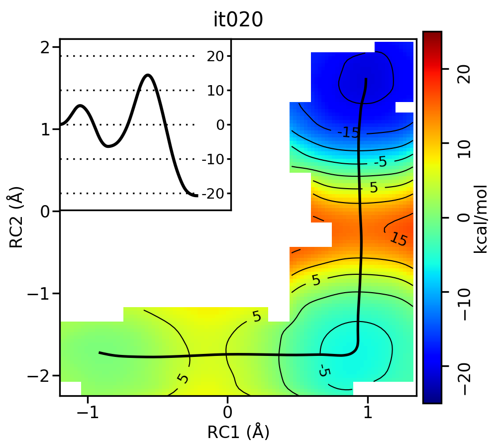
Take a look at the progression of the string by opening metafile.all.chk.wavg.0.path.png for the init, it002, it005, it010, and it020 directories.
For the linear guess, the progression looks something like this:
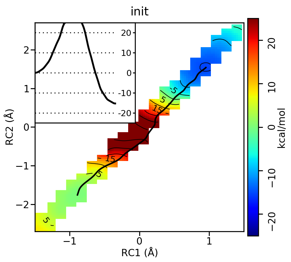
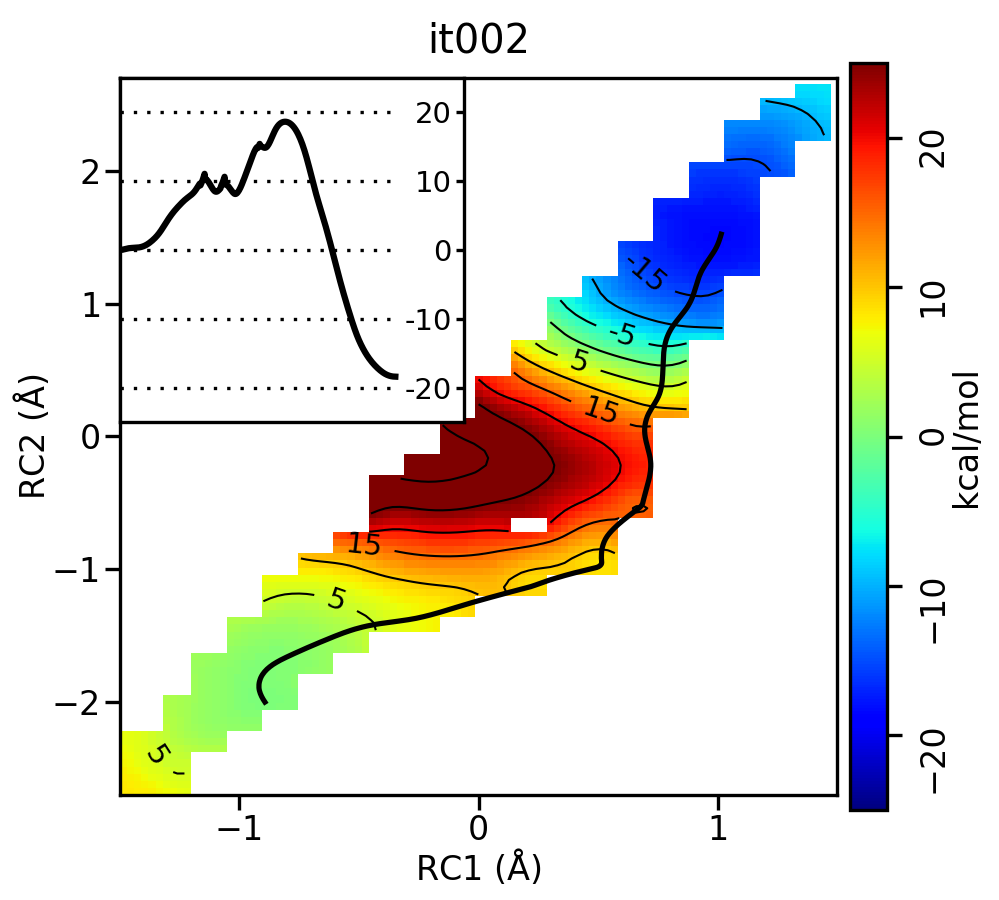
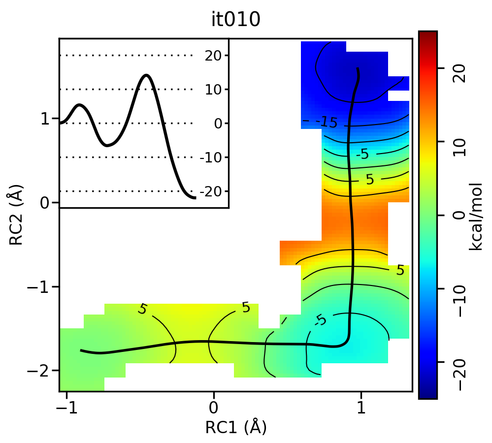

Figure 9. Free energy surfaces starting from a linear initial guess with optimized minimum free energy path (black) after iterations 0, 2, 5, 10, and 20. The inset shows the corresponding PMF.
Now let’s compare the path from the different starting guessed. Here is an example of the result from it020 of the strings initiated from the 3 different pathways:
Linear pathway
Stepwise (PT) pathway
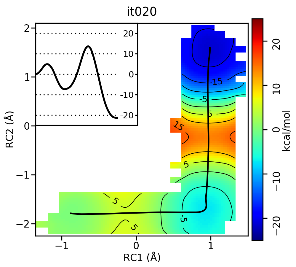
Stepwise (MT) pathway
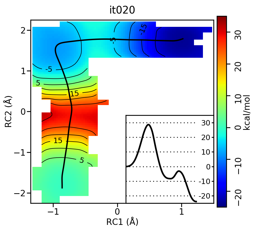
Figure 10. Free energy surfaces starting from a linear and two different step-wise initial guesses with optimized minimum free energy path from 20 string iterations (black). The inset shows the corresponding PMF.
We see that both the linear and stepwise initial guess where proton transfer (RC1) precedes methyl transfer (RC2) both converge to the minimum free energy path, but the stepwise initial guess where methyl transfer precedes proton transfer remains in that local minimum. This highlights that while the SASM is robust, like all string methods one should make educated, and potentially mulitple, initial guesses.