Soft-Core Potentials in Relative Binding Free Energy Calculations

Zeke A. Piskulich¹, Patricio Barletta¹, Ryan Snyder¹, and Darrin M. York¹

¹Laboratory for Biomolecular Simulation Research, Institute

for Quantitative Biomedicine and Department of Chemistry and Chemical

Biology, Rutgers University, Piscataway, NJ 08854, USA

Learning objectives

• Learn how soft-core potentials are formulated in Amber

• Describe the origin of end-point catastrophes, and how smoothstep soft-core potentials help avoid them

• Understand the impact of linear, soft-core, and smoothstep soft-core potentials on RBFE calculations.

Introduction to Soft-Core Potentials

In Absolute and Relative Binding Free Energy (RBFE) calculations, one of the key steps is to alchemically disappear a ligand (or transform a ligand into another ligand in the case of RBFE). Thus, to do this, we need to describe how that alchemical transformation will occur, in terms of how the atoms within the TI region’s interactions will be decoupled as a function of lambda. For this purpose, we use soft-core potentials, which are lambda dependent, to ensure that interactions are decoupled smoothly and to avoid singularities during the alchemical transformation.

In the following activity, please download the Jupyter Notebook and follow along.

Potential Energies in Amber

Recall, in a molecular simulation the potential energy of the system is described roughly by the following three equations:

\[ \begin{align}\begin{aligned}U_{LJ}=4\epsilon\left[\left(\frac{\sigma}{r}\right)^{12}-\left(\frac{\sigma}{r}\right)^{6}\right]\\U_{Coul}=\frac{1}{4\pi\epsilon_0}\frac{q_iq_j}{r}\\U_{dir}(r)=\frac{1}{4\pi\epsilon_0}\frac{q_iq_j\textrm{erfc}(\kappa r)}{r}\end{aligned}\end{align} \]

Where \(U_{LJ}\) is the Lennard-Jones potential, \(U_{Coul}\) is the Coulomb potential, and \(U_{dir}\) is the direct space part of the Ewald summation for electrostatics. In a soft-core potential, these equations are modified to include lambda dependent terms that ensure smooth decoupling of interactions as lambda goes from 0 to 1.

The core of the problem is that as a ligand is decoupled from the system, the interactions between the ligand and the rest of the system can become singular (i.e. go to infinity) as the ligand’s atoms are turned off.

Note

In this tutorial, we will be considering a radial pair of atoms that are being decoupled, but the same principles apply to fully decoupling a ligand as well (however, this would include more atoms in the soft-core region and require scaling of bonds, angles, and torsions as well).

Let’s first consider the simplest way of decoupling interactions, by simply scaling the interactions by lambda. In this case, the potential energy of the system would be described by the following equations:

\[U_{LJ}(r,\lambda)=(1-\lambda)U_{LJ}(r)\]

In Python, this would look like:

# Sigma, Epsilon, and kT are all set to reduced units for simplicity
sigma, epsilon, kT = 1.0, 1.0, 1.0
beta = 1.0/kT

def U_LJ(r):
    return 4*epsilon*((sigma/r)**12-(sigma/r)**6)

def U_linear(r, lam):
    return (1-lam)*U_LJ(r)

print("U_LJ at r=0.3 sigma:", U_LJ(0.3))
print("U_linear at r=0.3 sigma and lambda=0.5:", U_linear(0.3, 0.5))
print("U_linear at r=0.3 sigma and lambda=0.9:", U_linear(0.3, 0.9))

U_LJ at r=0.3 sigma: 7521218.7241857555
U_linear at r=0.3 sigma and lambda=0.5: 3760609.3620928777
U_linear at r=0.3 sigma and lambda=0.9: 752121.8724185753

As you can see, at low values of the separation distance (r) the potential energy explodes to very high values because its high up on the repulsive wall of the Lennard-Jones potential. With a linear scaling of the interactions, as lambda goes to 1, the potential energy will still be very high at low values of r, which can lead to poor convergence and sampling issues in the alchemical transformation.

Soft-Core Potentials

To avoid this issue, we use soft-core potentials which modify the equations for the potential energy to include lambda dependent terms that ensure smooth decoupling of interactions. The traditional soft-core potential for the Lennard-Jones interactions replaces the separation distance (r) with a modified separation distance (r’) that includes lambda dependent terms. The equations for the soft-core potential are as follows:

\[ \begin{align}\begin{aligned}r'_{LJ}=\left[r^n+\alpha\lambda\sigma^n\right]^{1/n}\\r'_{Coul}=\left[r^n+\beta\lambda\right]^{1/m}\end{aligned}\end{align} \]

Where n=6 and m=2 were traditionally used in older forms of the soft-core potential that are no longer recommended (see below), and alpha and beta are soft-core parameters that control the shape of the soft-core potential. The potential energy of the system is then calculated using these modified separation distances.

In Python, this would look like:

def rstar_trad(r, lam, alpha=0.5, n=6):
    return (r**n + alpha*lam*sigma**n)**(1.0/n)

print("Modified separation distance at r=0.3 sigma and lambda=0.5:", rstar_trad(0.3, 0.5))
print("Modified separation distance at r=0.3 sigma and lambda=0.9:", rstar_trad(0.3, 0.9))

Modified separation distance at r=0.3 sigma and lambda=0.5: 0.7940857966009571
Modified separation distance at r=0.3 sigma and lambda=0.9: 0.8756272130490854

As you can see, the modified separation distance (r’) is larger than the original separation distance (r) at low values of r and high values of lambda, which helps to avoid the singularity in the potential energy and allows for smoother decoupling of interactions during the alchemical transformation.

Smooth-Step Soft-Core Potentials

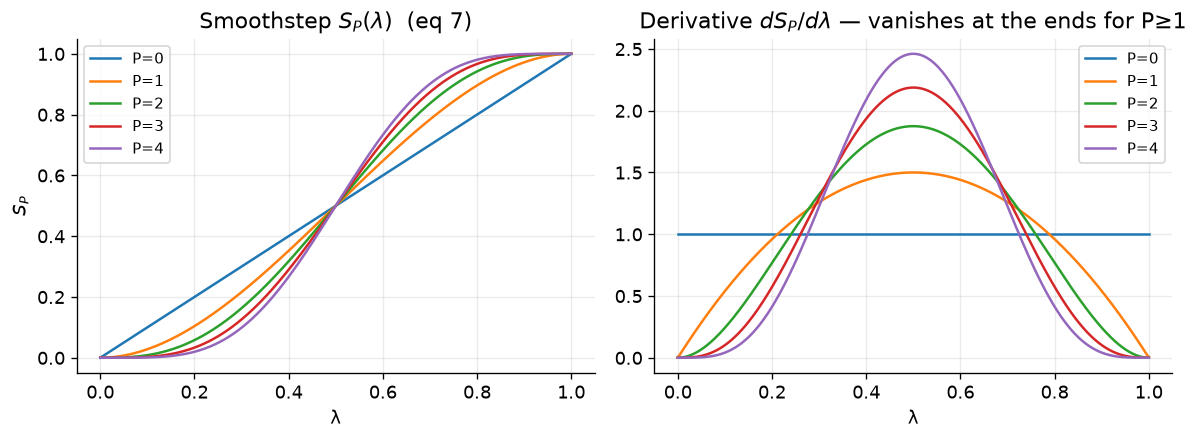
Now, there are some problems with the traditional soft-core potential, such as the fact that \(\alpha\) and \(\beta\) are set independently, which can lead to a mismatch in the decoupling of the Lennard-Jones and Coulomb interactions. Since the short-range repulsive barrier from the Lennard-Jones potential is what keeps particles from collapsing, if that is decoupled faster than the Coulomb interaction it can lead to particle collapse. To address this issue, we use second-order smoothstep functions to ensure that the Lennard-Jones and Coulomb interactions are decoupled in a more consistent manner Tsai et al.[1].

\[ \begin{align}\begin{aligned}S_P(\lambda) = \sum_{k=0}^P \binom{P+k}{k}\binom{2P+1}{P-k}\lambda^{P+k}(1-\lambda)^{P-k}\\S_1(\lambda) = 3\lambda^2 - 2\lambda^3\\S_2(\lambda) = 6\lambda^5 - 15\lambda^4 + 10\lambda^3\\S_3(\lambda) = -20\lambda^7 + 70\lambda^6 - 84\lambda^5 + 35\lambda^4\\S_4(\lambda) = 70\lambda^9 - 315\lambda^8 + 540\lambda^7 - 420\lambda^6 + 126\lambda^5\end{aligned}\end{align} \]

def S(x, P):
    x = np.clip(x, 0, 1)
    return {0: x,
            1: 3*x**2 - 2*x**3,
            2: 6*x**5 - 15*x**4 + 10*x**3,
            3: -20*x**7 + 70*x**6 - 84*x**5 + 35*x**4,
            4: 70*x**9 - 315*x**8 + 540*x**7 - 420*x**6 + 126*x**5}[P]

S2 = lambda x: S(x, 2)


x = np.linspace(0, 1, 400); dx = x[1]-x[0]

fig, ax = plt.subplots(1, 2, figsize=(10, 3.8))

# Make the Left Hand Figure
for P in range(5): ax[0].plot(x, S(x, P), label=f"P={P}")
ax[0].set_title("Smoothstep $S_P(\\lambda)$  (eq 7)"); ax[0].set_xlabel("λ"); ax[0].set_ylabel("$S_P$"); ax[0].legend(fontsize=9)

# Make the Right Hand Figure

for P in range(5): ax[1].plot(x, np.gradient(S(x, P), dx), label=f"P={P}")
ax[1].set_title("Derivative $dS_P/d\\lambda$ — vanishes at the ends for P≥1"); ax[1].set_xlabel("λ"); ax[1].legend(fontsize=9)

fig.tight_layout(); plt.show()

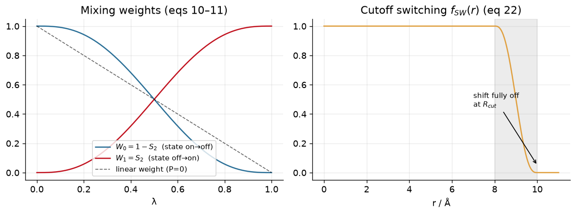
Now, we use these soft-core functions in two ways in an alchemical transformation. The first way is to use the soft-core function as a weight to mix the energy terms of the two end states.

This is defined as follows:

\[ \begin{align}\begin{aligned}W_0(\lambda) = 1 - S_P(\lambda)\\W_1(\lambda) = S_P(\lambda)\end{aligned}\end{align} \]

where \(W_0\) and \(W_1\) are the weights for the two end states, and \(S_P(\lambda)\) is the smoothstep function of order P. The potential energy of the system is then calculated as a weighted sum of the potential energies of the two end states, with the weights appearing and leaving with zero derivatives at the endpoints of lambda.

A switching function is also used to recover the true value of r at the nonbonded cutoff, which is defined as follows:

\[f_{SW}(r)=1-S_2\left(\frac{r-R_{cut,i}}{R_{cut,f}-R_{cut,i}}\right)\]

where here, \(R_{cut,i}\) is the distance at which the soft-core potential begins to switch to the true potential, and \(R_{cut,f}\) is the distance at which the soft-core potential fully switches to the true potential. This switching function ensures that the potential energy of the system transitions smoothly from the soft-core potential to the true potential as the separation distance (r) approaches the nonbonded cutoff.

def f_SW(r, Rci, Rcf):
    return 1.0 - S2(np.clip((r - Rci)/(Rcf - Rci), 0, 1))    # eq 22

fig, ax = plt.subplots(1, 2, figsize=(10, 3.8))

ax[0].plot(x, 1-S2(x), color=C["new"], label="$W_0=1-S_2$  (state on→off)")
ax[0].plot(x, S2(x),   color=C["lin"], label="$W_1=S_2$  (state off→on)")
ax[0].plot(x, 1-x, "k--", lw=1, alpha=.6, label="linear weight (P=0)")
ax[0].set_title("Mixing weights (eqs 10–11)"); ax[0].set_xlabel("λ"); ax[0].legend(fontsize=9)

rr = np.linspace(0, 11, 400); Rci, Rcf = 8.0, 10.0

ax[1].plot(rr, f_SW(rr, Rci, Rcf), color=C["trad"]); ax[1].axvspan(Rci, Rcf, color="grey", alpha=.15)
ax[1].set_title("Cutoff switching $f_{SW}(r)$ (eq 22)"); ax[1].set_xlabel("r / Å")
ax[1].annotate("shift fully off\nat $R_{cut}$", (10, 0.05), (7.0, 0.45), fontsize=9, arrowprops=dict(arrowstyle="->"))

fig.tight_layout(); plt.show()

These smoothstep soft-core potentials are then used to generate a new set of modified distances.

\[ \begin{align}\begin{aligned}r'_{LJ} = \left[r^n + \alpha_{LJ}\sigma_{ij}^nS_2(\lambda)f_{SW}(r)\right]^{1/n}\\r'_{Coul} = \left[r^m + \alpha_{Coul}\sigma_{ij}^mS_2(\lambda)f_{SW}(r)\right]^{1/m}\end{aligned}\end{align} \]

We can define these in python as:

def rstar_new(r, lam, alpha=0.5, n=2, switch=False, Rci=8.0, Rcf=10.0):
    fsw = f_SW(r, Rci, Rcf) if switch else 1.0
    return (r**n + alpha*(sigma**n)*S2(lam)*fsw)**(1.0/n)

print("Modified separation distance at r=0.3 sigma and lambda=0.5:", rstar_new(0.3, 0.5))
print("Modified separation distance at r=0.3 sigma and lambda=0.9:", rstar_new(0.3, 0.9))

Modified separation distance at r=0.3 sigma and lambda=0.5: 0.58309518948453
Modified separation distance at r=0.3 sigma and lambda=0.9: 0.7653234610280811

So now, let’s compare what the potential energy looks like for a linear scaling of the interactions, the traditional soft-core potential, and the new smoothstep soft-core potential.

# coupled potentials for a disappearing LJ particle

def U_trad(r, lam, alpha=0.5):                                # eqs 18 + 23, linear weight
    return (1.0 - lam)*U_LJ(rstar_trad(r, lam, alpha))

def U_new(r, lam, alpha=0.5):                                 # eqs 20 + 23, smoothstep weight
    return (1.0 - S2(lam))*U_LJ(rstar_new(r, lam, alpha))

# Plot: the infinite wall at r->0 becomes a finite hill as the particle vanishes
r = np.linspace(0.001, 2.2, 2000)

fig, ax = plt.subplots(1, 3, figsize=(10, 4.0))

for lam in [0.0, 0.4, 0.7, 0.95]:
    ax[0].plot(r, U_linear(r, lam), label=f"λ={lam}")
    ax[1].plot(r, U_trad(r, lam), label=f"λ={lam}")
    ax[2].plot(r, U_new(r, lam),  label=f"λ={lam}")

for a, t in zip(ax, ["Linear", "Traditional Soft-Core", "Smooth-Step Soft-Core)"]):
    a.set_ylim(-1.5, 8); a.set_xlim(0, 2.2); a.set_title(t, fontsize=10.5)
    a.set_xlabel(r"r / $\sigma$"); a.axhline(0, color="k", lw=.6, alpha=.5); a.legend(fontsize=9)

ax[0].set_ylabel(r"U(r; λ) / $\epsilon$")

fig.suptitle("A disappearing particle (λ: 0→1): the hard wall at r→0 becomes finite", fontsize=11)
fig.tight_layout(); plt.show()

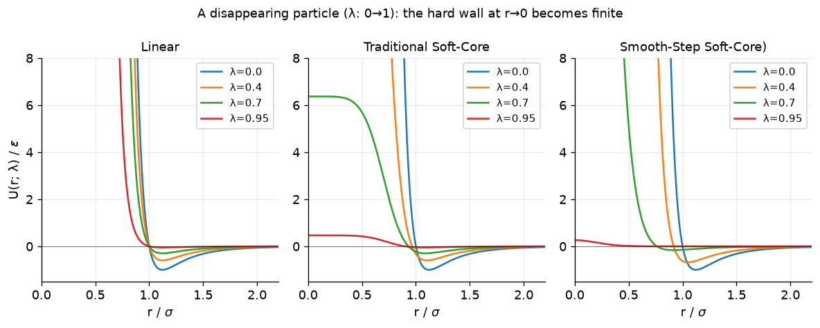
In the above plots, we compare the three scaling approaches. Clearly, in the linear scheme as small separation distances the value of the potential still explodes. The traditional soft-core and smooth-step approaches solve the explosion problem. So why the smoothstep?

Let’s consider what happens in an alchemical transformation. For our 1-D radial pair model, the TI average at a fixed \(\lambda\) is a Boltzmann-weighted integral over the separation (with a 3D volume element \(g(r)=4\pi r^2\)).

\[\left\langle\frac{\partial U}{\partial \lambda}\right\rangle_\lambda = \frac{\int g(r) \frac{\partial U}{\partial \lambda} e^{-\beta U(r,\lambda)} dr}{\int g(r) e^{-\beta U(r,\lambda)} dr}\]

We can examine this integral for the three cases.

def moments(Ufun, lam, r_min=0.02, R_box=2.5, N=400000, h=1e-5):

    # Return <DU/DL> and Var(DU/DL) for the 1-D radial pair model at fixed lambda.
    r = np.linspace(r_min, R_box, N)
    g = 4*np.pi*r**2
    w = g*np.exp(-beta*Ufun(r, lam))                 # Boltzmann weight x volume element
    Z = np.trapz(w, r)
    lo, hi = max(lam-h, 0.0), min(lam+h, 1.0)
    dUdl = (Ufun(r, hi) - Ufun(r, lo))/(hi - lo)     # central finite difference
    m1 = np.trapz(w*dUdl, r)/Z
    m2 = np.trapz(w*dUdl*dUdl, r)/Z
    return m1, m2 - m1*m1

lams = np.linspace(0, 0.985, 40)

I = {nm: np.array([moments(f, l) for l in lams])
     for nm, f in [("lin", U_linear), ("trad", U_trad), ("new", U_new)]}

fig, ax = plt.subplots(figsize=(7, 4.2))
ax.plot(lams, I["lin"][:,0],  color=C["lin"],  lw=2, label="linear (no soft-core)")
ax.plot(lams, I["trad"][:,0], color=C["trad"], lw=2, label="traditional soft-core")
ax.plot(lams, I["new"][:,0],  color=C["new"],  lw=2, label="new smoothstep soft-core")
ax.axhline(0, color="k", lw=.6); ax.set_xlabel("λ")
ax.set_ylabel(r"$\langle \partial U/\partial\lambda\rangle_\lambda$  /  ε")
ax.set_title("TI integrand: linear coupling plunges near λ→1 (end-point catastrophe)")
ax.legend(fontsize=9.5); fig.tight_layout(); plt.show()

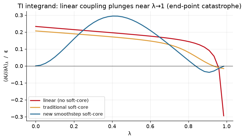
Note the end-point catastrophe that we get with a linear schedule at \(\lambda = 1\). Meanwhile, a traditional soft-core potential performs better (but is still non-zero at the end points). Finally, the new smoothstep soft-core potential approaches both end-points with zero slope.

Note

The recommended values of n and m are n=2 and m=2. Likewise, the suggested values are \(\alpha_{LJ}=0.5\) and \(\alpha_{Coul}=1.0\).

Using Soft-Core Potentials in Amber

In the Amber Molecular Dynamics package, we define Soft-Core Potentials through the following parameters:

• ifsc=1: Turns on soft-core potentials. These by default reflect the “traditional” soft-core potentials described above.

• gti_lam_sch=1: Replaces \(\lambda\) with \(S_P(\lambda)\)

• scalpha: Sets the \(\alpha\) term for the soft-core potentials

• scbeta: Sets the \(\beta\) term for the soft-core potentials

• gti_scale_beta=1: Sets the soft-core potentials to match the functional form described above for the smoothstep soft-core potentials (but doesn’t include smoothing at the non-bonded cutoff). (Also sets scalpha=0.5, scbeta=1.0)

• gti_vdw_exp=2: Sets the n parameter for the exponent. (Note - the default is 6).

• gti_elec_exp=2: Sets the m parameter for the exponent.

• gti_cut_sc=2: Adds the smoothing to the non-bonded cutoff (the \(f_{SW}(r)\) term above)

The lambda schedule is controlled by the file lambda.sch, which looks as follows:

Warning

The Amber Manual currently incorrectly states the defaults for the lambda.sch files. Below are the current actual default values.

TypeGen, smooth_step2, complementary, 0.0, 1.0
TypeBAT, smooth_step2, complementary, 0.0, 1.0
TypeEleRec, smooth_step2, complementary, 0.0, 1.0
TypeEleCC, smooth_step2, complementary, 0.0, 1.0
TypeEleSC, smooth_ step2, complementary, 0.0, 1.0
TypeVDW, smooth_ step2, complementary, 0.0, 1.0

Warning

Your selected parameters for the smoothstep soft-core potentials can significantly impact the stability of your calculations.

Recommended parameter choices are:

gti_vdw_exp=2 gti_elec_exp=2 gti_scale_beta=1 (which sets scalpha=0.5, scbeta=1) and to use the smooth_step2 lambda schedule for the lambda.sch file as shown in the code-block above.

The full comparison of our best-practices compared to defaults is included below.

+------------------+--------+---------------------------+---------------------------+
| Parameter        | Ours   | gti_lam_sch==0            | gti_lam_sch==1            |
+------------------+--------+---------------------------+---------------------------+
| gti_cut_sc       | 2      | 0                         | 0                         |
| gti_ele_exp      | 2      | 2                         | 2                         |
| gti_vdw_exp      | 2      | 6                         | 6                         |
| gti_ele_sc       | 1      | 0                         | 1                         |
| gti_vdw_sc       | 1      | 0                         | 1                         |
| scalpha          | 0.5    | 0.5                       | 0.2                       |
| scbeta           | 1.0    | 12.0                      | 50.0                      |
| gti_auto_alpha   | N/A    | 0                         | 0                         |
+------------------+--------+---------------------------+---------------------------+

You can download an example Amber soft-core input set here: tyk2_softcore.tar.gz

Now let’s try this out. First, download the above tar archive, and then decompress it.

tar -xvf tyk2_softcore.tar.gz
cd tyk2_softcore

In this directory, you will find a parm7 and rst7 file for ejm31, a ligand for Tyk2, in vacuum, along with a sample mdin file (and a script run.sh which runs pmemd.cuda on it).

Let’s start off by running the file. If you look at the parameters above, you can see that we’ve put in place the second-order smoothstep soft-core potential for you to try. Note that clambda=1.0 in this example so that we can see the difference the parameters make.

When you run it, take a look at DU/DL in the produced mdout. You’ll see DU/DL is zero - which is what we expect from the above tutorial.

Let’s switch it up, however. What if we change the settings a bit and revert to traditional soft-core potentials?

cp sp_lam_1.0.mdin ts_lam_1.0.mdin

Edit this file so that the section following clambda looks as follows.

ifsc = 1,
timask1 = ':LIG',
scmask1 = ':LIG',
timask2 = '',
scmask2 = '',
scalpha = 0.5,
scbeta = 1.0,
gti_add_sc = 25,
gti_scale_beta = 0,
gti_lam_sch = 0,

What happened to dU/dL at the endpoint? Note that the DU/DL is no longer zero at the end-point. This is not ideal!

Finally, let’s fully revert to linear scaling.

ifsc = 0,
timask1 = ':LIG',
timask2 = ':LIG',
gti_scale_beta = 0,
gti_lam_sch = 0,

This again gives a DU/DL value that is significantly different from 0.

Take some time to modify parameters (for instance the soft-core parameters in the original smoothstep mdin) to get a feel for how they modulate the behavior. What breaks behavior at the end-point? Also, take some time to look at the entries for the soft-core region in the mdout.

Note

In this final example, gti_add_sc=25 was used which also scales torsions and angles (further scope than the rest of this activity). For more information, please refer to the Amber manual.

Relevant Literature

[1]

Hsu-Chun Tsai, Tai-Sung Lee, Abir Ganguly, Timothy J Giese, Maximilian Ccjc Ebert, Paul Labute, Kenneth M Merz Jr, and Darrin M York. AMBER Free Energy Tools: A New Framework for the Design of Optimized Alchemical Transformation Pathways. J. Chem. Theory Comput., 19:640–658, 2023.