Exploring FE-Toolkit HTML Edge Reports

Zeke A. Piskulich¹, Timothy Giese¹, Patricio Barletta¹, Ryan Snyder¹, and Darrin M. York¹

¹Laboratory for Biomolecular Simulation Research, Institute

for Quantitative Biomedicine and Department of Chemistry and Chemical

Biology, Rutgers University, Piscataway, NJ 08854, USA

Learning objectives

• Interpret an Edgembar HTML edge report for a real Tyk2 ABFE calculation.

• Diagnose simulation quality from the report’s error and warning metrics (equilibration, statistical inefficiency, phase-space overlap).

• Compare BAR vs. TI estimates and inspect the convergence, dV/dL, and replica-exchange plots to judge whether a calculation is trustworthy.

Activities

In this Activity, you will learn how to explore HTML edge reports generated with FE-Toolkit. This tutorial will guide you through the process of interpreting the various plots and tables included in the HTML report, and how to use this information to assess the quality of your free energy calculations.

FE-Toolkit HTML Reports

For this tutorial, we have provided the simulation output data from Absolute Binding Free Energy Calculations on Tyk2 for four ligands. In this tutorial, we will primarily use the files for the ligand ejm31; however, we have provided the other ligands as a reference (and as an opportunity for further practice).

The HTML report can be viewed here: Graph.html

Header

Hint

** Troubleshooting Questions **

1. Do you have many errors and warnings?

2. Are you using a recent hash of edgembar?

The first thing you see in an HTML report is the header. It contains important information about the calculation, specifically which version of edgembar was used, what command called edgembar, and what errors and warnings were generated.

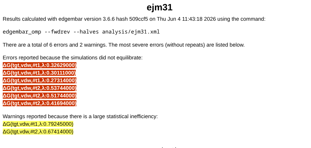
A few things are worth pointing out: every version of edgembar is given a unique hash (in the above image 3.6.6 H09ccf5), which can be useful for debugging.

Next, a summary of errors (shown in red) and warnings (shown in yellow) is included. Each entry is a hyperlink that jumps to the trial and lambda window where the issue was detected. These errors and warnings correspond to a few different aspects of a simulation’s quality. MOre details on the test that edgembar perfomrs to determine these errors and warings are availabe at FE-Toolkit edgembar guide: edgembar edge analysis.

• Equilibration — whether too much of the simulation had to be discarded before reaching a stable production region. A simulation is flagged as unequilibrated if the discarded fraction exceeds --fmaxeq (default 0.5, i.e. 50%). In the report, this appears in the <f_eq> (fraction discarded) and N_eq (number of equilibration samples) columns of the per-trial data tables, and the convergence status is shown in the Conv? column.

• Statistical inefficiency — how strongly correlated the samples in the production region are (larger is worse). A warning is raised if it exceeds 50; an error if it exceeds 100. In the report, this is the <g_prod> column (with g_ana for the analysis region and g for all data) of the per-trial data tables.

• Number of independent samples — how many statistically independent samples remain in the production region (fewer is worse). This is computed as the number of samples divided by the statistical inefficiency. A warning is raised if there are fewer than 100; an error if there are fewer than 50. In the report, this is the N_ana column (with N for all data) of the per-trial data tables.

• Phase-space overlap — how well a lambda window overlaps with its next neighbor (lower is worse). A warning is raised if the overlap is less than 0.25; an error if it is less than 0.15. In the report, this is the S column of the per-trial data tables.

• Reweighting entropy — the effective sampling overlap with the next neighboring window (lower is worse). A warning is raised if it is less than 0.6; an error if it is less than 0.4. In the report, this is the RE column of the per-trial data tables.

How the production region is identified — and therefore which simulations get flagged as unequilibrated — can be tuned with the following analysis options to edgembar:

• --ptol — the significance level (p-value) for the test that detects the production region. Larger values discard more data as equilibration.

• --dtol — if the first-half and last-half means are within this tolerance (default: 0.1 kcal/mol), the window is treated as equilibrated.

• --fmaxeq — the maximum fraction of a simulation that may be discarded as equilibration (default: 0.5).

• --ferreq — flag a simulation as an error if more than this fraction would be discarded (default: equal to --fmaxeq).

• --no-auto — disable automatic equilibration detection entirely and analyze all samples from --fstart to --fstop.

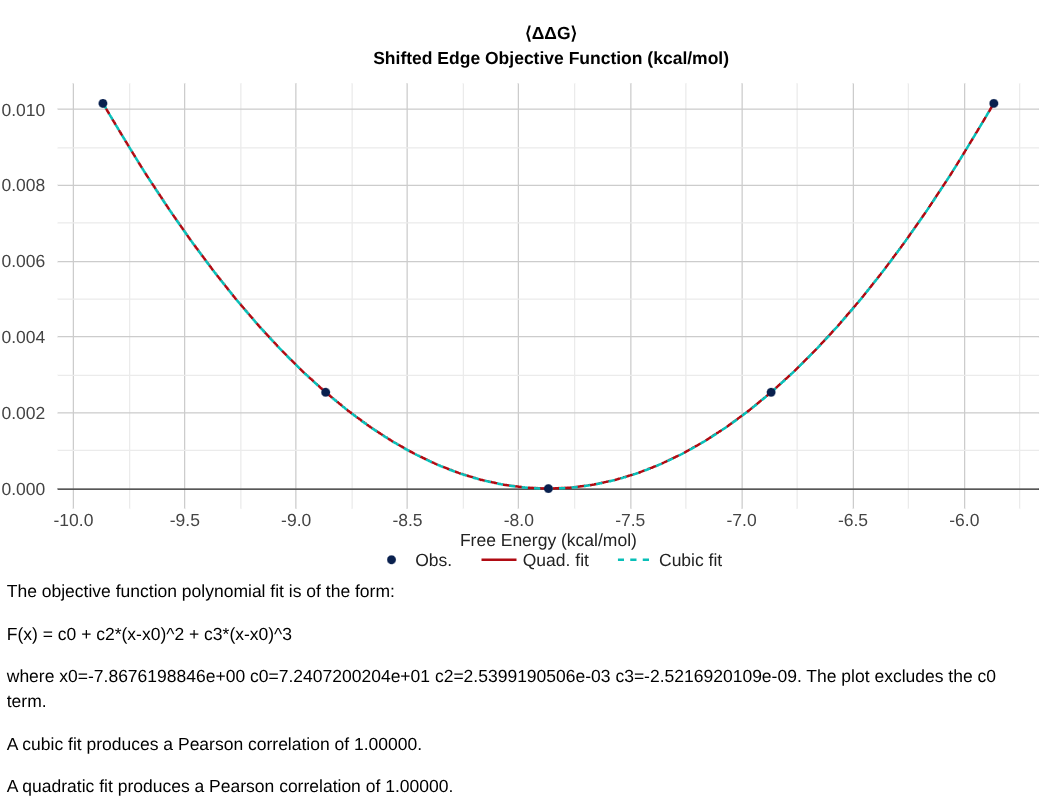
Objective Function

The next plot you see in the edge report is the “Shifted Edge Objective Function”, which shows the objective function that was minimized across all samples of an edge to obtain a specific final value shown on the x-axis. The minimum value corresponds to an unconstrained variational solution of the MBAR or BAR equations. Other values correspond to constrained variational solutions (where the constraint is for the x-axis value).

Unless there are problems with the simulation data, this plot should be a quadratic function that can be pre-computed for each edge and used to efficiently solve the network-wide set of equations. The curve is fit to a quadratic and cubic function using the 5 points indicated. These fits should produce Pearson correlations greater than 0.99, and the cubic terms should be less than \(10^{-5}\).

Note

The edge objective function is only relevant for network-wide analysis; it does not affect any aspect of the edge report. The edgembar-WriteGraphHtml.py script performs network-wide analysis, and by default solves for the node free energies using a quadratic approximation for the edge objective functions. This is often sufficient. One can use --solver=nonlinear or --solver=mixed to solve with the cubic fits. The mixed version solves with the cubic fits but then does bootstrap error calculations using the quadratic fits. This --solver=nonlinear or --solver=mixed is not recommended because it is very slow and not necessarily more accurate unless there were severe discrepancies in the objective function fits shown in the edge report.

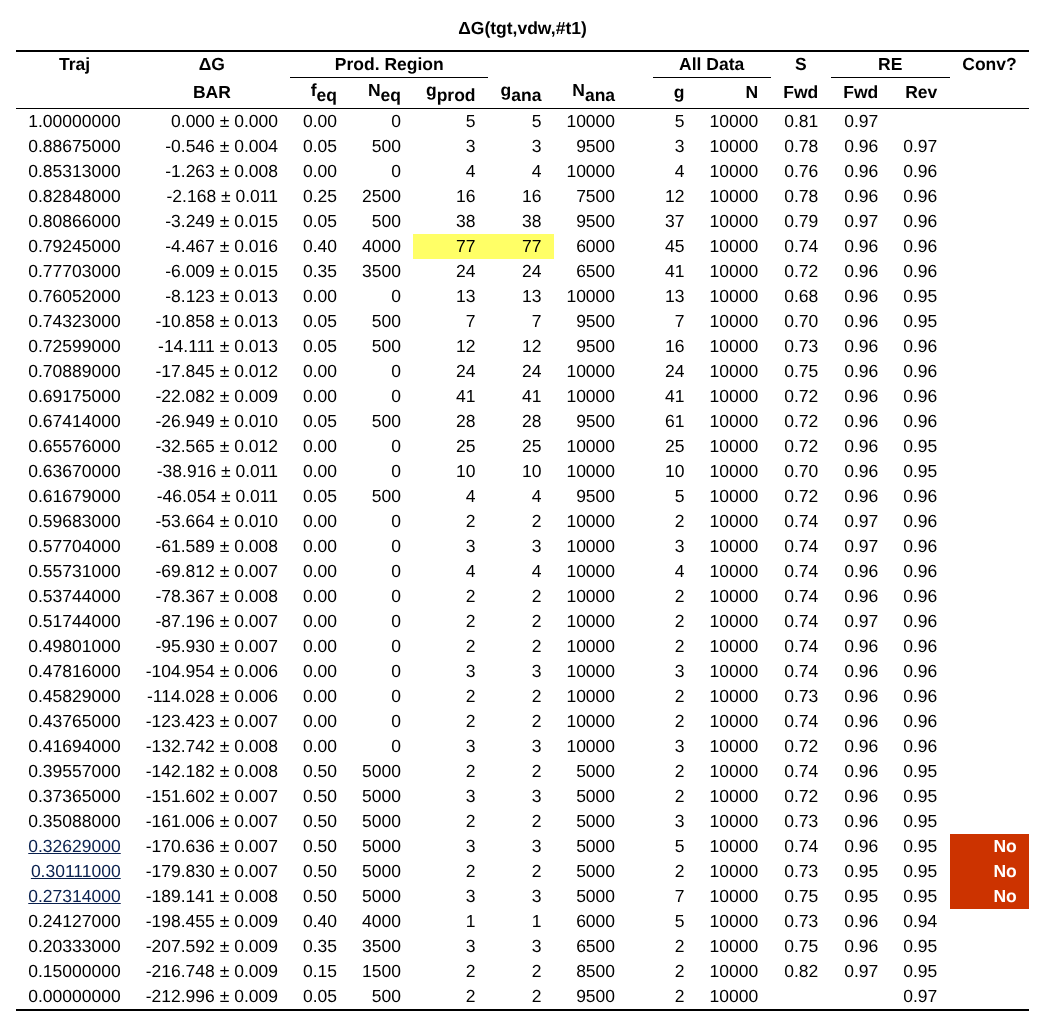
Overall results

Hint

** Troubleshooting Questions **

1. Do your BAR and TI results in the table agree?

2. How far does your fwdrev analysis deviate from production?

3. Is there a significant trend in your first and last half analysis?

The next set of data you’ll see is a summary table of the free energy values, and-if you ran edgembar with - -fwdrev and - -halves -a pair of timeseries figures above it. The “Fwd & Rev Analysis” figure shown on the left compares the free energies calculated from the first X% of the data to those calculated from the last X% of the data. The “First- & Last-Half Analysis” figure shown on the right which excludes X% of the simulation from start as equilibration, and splits the remaining 100-X% of data into two halves and compares the free energy from each half.

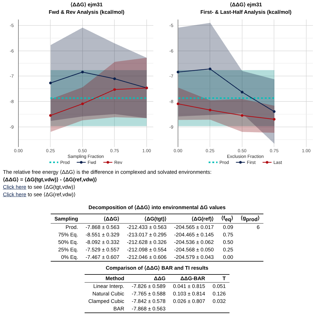
Most important is the table at the bottom, which gives you a summary of the values from analysis with Bennett’s Acceptance Ratio (BAR) [1], and Thermodynamic Integration (TI) [2].

Note

A key debugging tool is to check agreement between BAR and TI. If these values do not agree - it suggests a problem with either equilibration, replica exchange acceptances, or alchemical pathway.

The shaded bands around the lines are 95% confidence intervals, obtained by scaling the standard error of the mean by 1.96 - a factor that tends to underestimate the true confidence interval. When the fwdrev or halves lines separate from each other by more than these bands, it usually points to a problem with the simulation or its equilibration. In that situation, it helps to inspect the trajectory directly: the plots alone may not reveal whether the start of the simulation was insufficiently equilibrated or if something catastrophic happened in the middle to simulate it incorrectly near the end.

DV/DL Profiles and Replica Exchanges

Hint

** Troubleshooting Questions **

1. Is your DV/DL profile smooth? Does it have weird discontinuities?

2. Are there big differences in your DV/DL profiles between trials?

3. Does your replica exchange acceptance ratio ever approach a low number (< 0.2?)

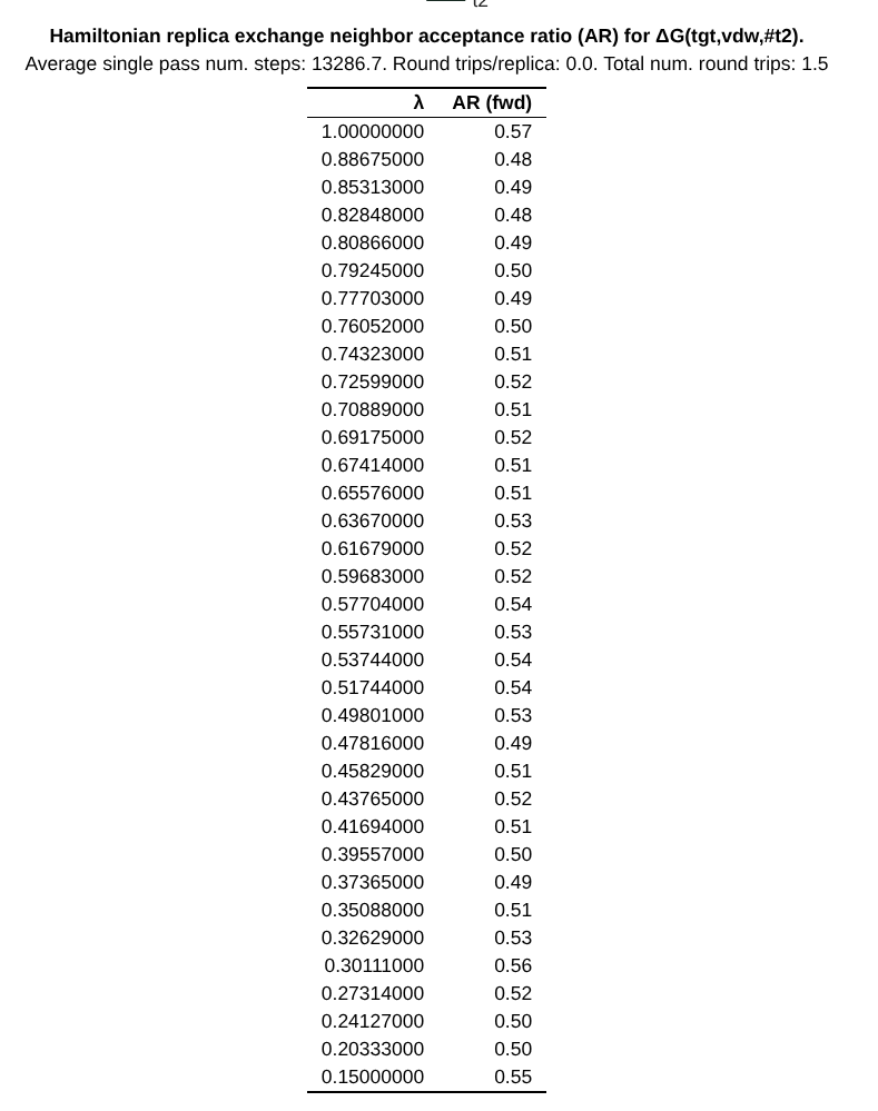
The next key set of plots that are found are the DV/DL profile, and the Replica Exchange Acceptance Ratios.

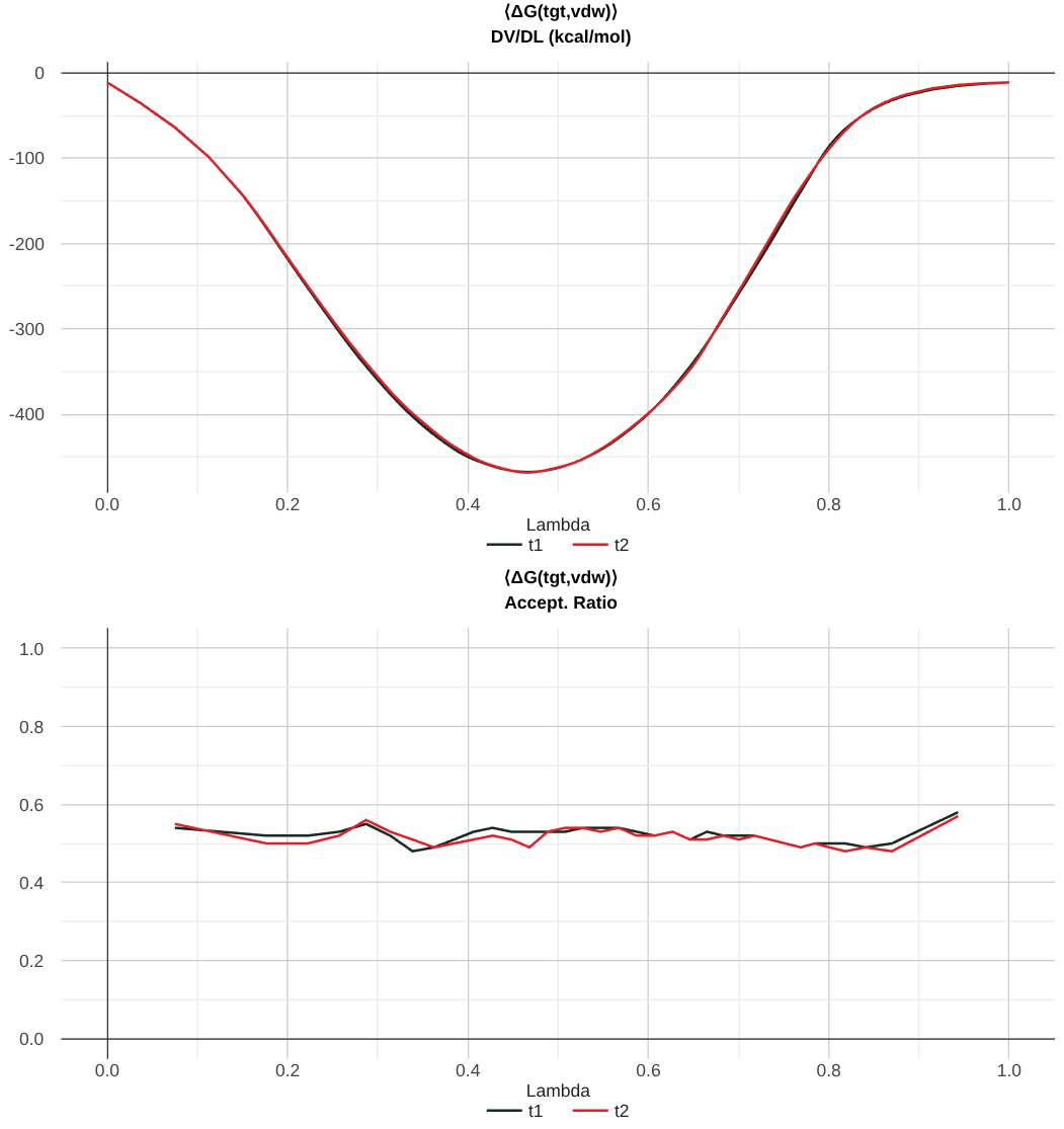
In the above image, you can see a well-converged DV/DL profile. Note that the trials track pretty well along each other.

Recall that the dV/dL profile is intrinsically linked to the free energy by the equation:

\[\Delta G = \int_0^1 \left\langle \frac{\partial V(\mathbf{x}; \lambda)}{\partial \lambda} \right\rangle_{\lambda} d\lambda\]

Note

For ABFE calculations, the dV/dL profile is shifted by a constant number. This number originates from the correction to the free energy that comes from Boresch Restraints. Determining the Boresch Restraint Contribution to the Free Energy.

Now, the replica exchange acceptance ratio is included in the second plot, and it gives you information for each pair of lambda windows what percentage of exchanges were accepted. Here, the value of 0.5 suggests that there were sufficient exchanges.

Data Tables

Hint

** Troubleshooting Questions **

1. Did a lot of simulation data get thrown out when selecting production regions?

2. Did this trial have many (or most) of the warnings?

3. Do you have single passes and round trips in your calculation?

The next major section of the file is a set of tables (per environment and per trial) that give summary information about the free energy calculation as a function of lambda.

The columns of this trial data table are separated into three sections that report the same statistics computed over different subsets of the data. One section reports the statistics computed using only the “production region” (columns ending in _prod, such as <g_prod>). Another section reports the statistics computed when “all data” is considered (columns such as g). The “ana” section (columns ending in _ana, such as g_ana) reports the statistics for the data that are actually being analyzed, which could be either the “all data” or the “production region” depending on the analysis options used.

There is also a replica exchange data table that provides the data included in the acceptance ratio plot.

The header of this table includes a few additional useful pieces of information:

• Average single pass num. steps: The amount of time it takes for a replica to exchange all the way \(0 \rightarrow 1\) or \(1 \rightarrow 0\)

• Round trips/replica: Total number of round trips divided by the number of replicas.

• Total num. round trips: The number of times a replica traverses \(0 \rightarrow 1 \rightarrow 0\) or \(1 \rightarrow 0 \rightarrow 1\)

Troubleshooting

Hint

** Troubleshooting Questions **

1. Does the window look converged?

2. What is the scale of the dependence on the y-axis of the block average

Each lambda window that has a warning also gets a special section which includes information about the convergence of that window.

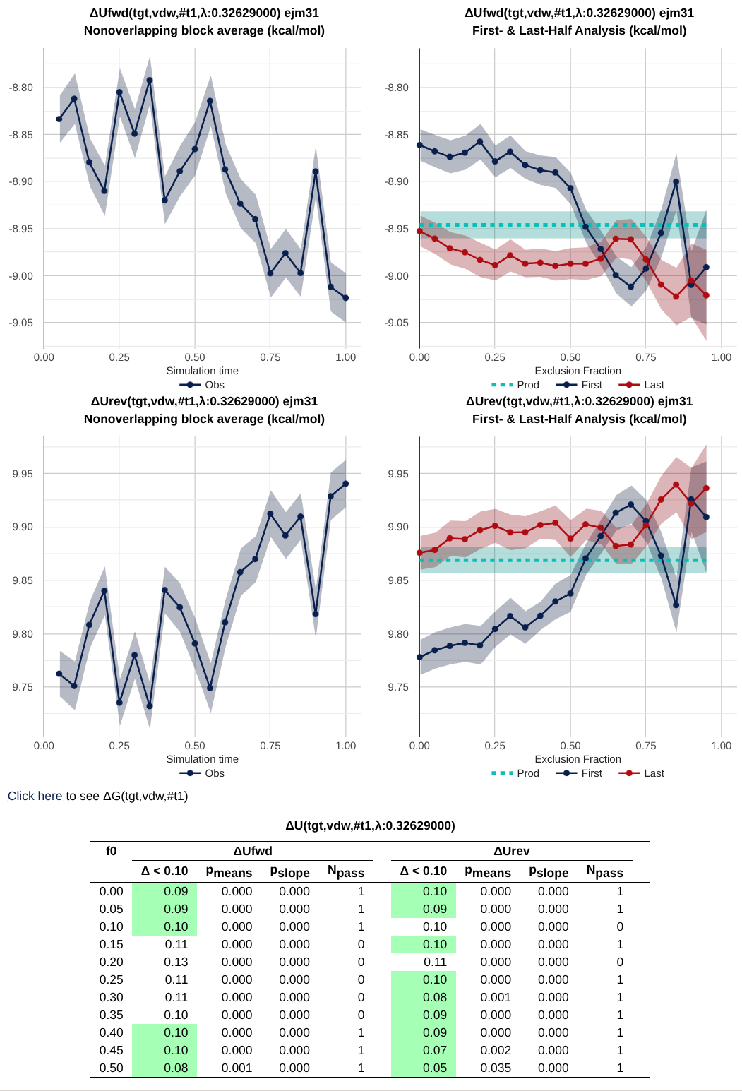
This shows plots of block averages over time, data tables, etc that can be used for additional debugging.

Wrapping Up

In this activity, you walked through the pieces of an HTML report. Go through the troubleshooting questions at the top of each relevant section with that report. Does this pass as an okay simulation?

Relevant Literature

[1]

Charles H. Bennett. Efficient estimation of free energy differences from Monte Carlo data. J. Comput. Phys., 22:245–268, 1976.

[2]

John G. Kirkwood. Statistical mechanics of fluid mixtures. J. Chem. Phys., 3:300–313, 1935.